Category Archives: Sports Science

Using Beta-Binomial Regression to Set Priors for Different Sample Sizes

In a prior post I explained an approach for using Bayes to estimate a player’s 3pt% based on prior knowledge of 3pt success in NBA players. This approach took advantage of the beta-binomial conjugate.

In that post, I constrained our analysis to only players that had 200 or more 3pt attempts during the course of a season. But, what if we don’t want to only focus on players that obtained a certain number of 3 point attempts? What about players who only took 100 attempts? 10 attempts? 2 attempts?! What can be said about their performance?

Today, we will discuss the approach of using beta-binomial regression to first establish a prior 3pt%, based on the number of 3pt attempts the player shot (sample size) and then update that prior based on the success that the player had in those attempts.

The code for this article is available on my GITHUB page.

A few references of books that I’ve found useful for building Bayesian models are at the end of this post. The approach here was inspired by Chapter 7 of David Robinson’s fantastic book, Introduction to Empirical Bayes: Examples from Baseball Statistics.

The Data

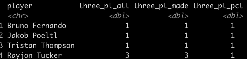
We will use the three point attempts data for all players in the 2022 NBA season. Data was scraped from basketball-reference.com. In total, there are 740 rows of data. Here is what the first four look like:

Plotting the Data

To help wrap our heads around the relationship between 3pt% and 3pt attempts, we will build a simple plot.

Notice that the number of 3 point attempts has some influence on 3pt%. First, as 3pt attempts increase, so does 3pt%. This is because better 3pt shooters will take more 3pt shots and, because they are good, their teams will also try and put them in position to take these shots.  Additionally, we can see that as 3pt attempts increase, the amount of variance in performance decreases. Players with under 100 3pt attempts are relatively spread out around the regression line.

Bayesian Shrinkage using the Beta-Binomial Conjugate

As a review from the prior blog article on this topic, we can use our knowledge of the 3pt% success of NBA players as a prior to help shrink observations towards the “expected” outcome. The amount of shrinkage a player exhibits will be dependent on the number of 3pt attempts they have. A smaller sample size means we have less confidence in the observed performance and thus greater shrinkage towards the population prior. Conversely, a large sample size means more confidence in the observed performance and therefore much less shrinkage.

From the prior article we estimated the alpha and beta parameters for our beta distribution to be 61.8 and 106.2, respectively. Recall that these values were estimated from the prior 2 seasons and using only those players with 200 or more 3pt attempts. The alpha and beta parameters provide us with a prior mean for NBA 3pt% of 36.8%.

We will apply this prior knowledge to the observations of all players in our 2022 data set by using the beta-binomial conjugate.

alpha <- 61.8
beta <- 106.2

prior_mu <- alpha / (alpha + beta)
prior_mu

tbl2022 <- tbl2022 %>%
  mutate(three_pt_missed = three_pt_att - three_pt_made,
         posterior_alpha = three_pt_made + alpha,
         posterior_beta = three_pt_missed + beta,
         posterior_three_pt_pct = posterior_alpha / (posterior_alpha + posterior_beta),
         posterior_three_pt_sd = sqrt((posterior_alpha * posterior_beta) / ((posterior_alpha + posterior_beta)^2 * (posterior_alpha + posterior_beta + 1))))


Next, we create a plot to see how the beta-binomial posterior for each player looks relative to the raw data (plotted on the left):


Combining our prior and observed values we can see (on the right) that the data are now constrained around the prior (36.8%). Players with a small number of observations (on the left) are pulled nearest to the line while players with larger observations (on the right) are less influenced by the prior and tend to remain closer to their observed performance.

The problem is that the prior mean (36.8%) is too high for the players with a small number of 3pt attempts. Surely we wouldn’t want to make the assumption that their performance is close to the prior for players that had over 200 attempts! For example, the players with under 50 attempts have an observed average 3pt% of 30% and a median 3pt% of 25% (just over 10% less than those those who had 200 or more attempts!).

To deal with this issue we need to account for shot attempts first so that we can estimate players with smaller sample sizes relative to a prior performance that is more appropriate for them (IE, a prior that is lower than that currently being assumed by our alpha and beta parameters).

Accounting for 3pt Shot Attempts

Our outcome variable is binomial (success and failures) so we will use a beta-binomial regression to estimate a prior for 3pt% while controlling for 3pt shot attempts.

suppressPackageStartupMessages({
  suppressWarnings({
    library(gamlss)
  })
})

fit_3pt <- gamlss(cbind(three_pt_made, three_pt_missed) ~ log(three_pt_att),
                  data = tbl2022,
                  family = BB(mu.link = "identity"))

## extract model coefficients
fit_3pt$mu.coefficients
fit_3pt$sigma.coefficients


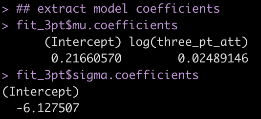
Now we can use these model coefficients to fit an estimated 3pt% for each player based on their number of 3pt attempts. This estimation will serve as our prior, which we will then turn into a new posterior 3pt% for each player using our beta-binomial approach. Note that while the mean 3pt% for each player will vary depending on shot attempts the population sigma will be constant for all athletes, representing the variance that we expect all of those in the population to similarly exhibit.

tbl2022 <- tbl2022 %>%
  mutate(mu = fitted(fit_3pt, parameter = "mu"),
         sigma = fitted(fit_3pt, parameter = "sigma"),
         prior_alpha_reg = mu / sigma,
         prior_beta_reg = (1 - mu) / sigma,
         posterior_alpha_reg = prior_alpha_reg + three_pt_made,
         posterior_beta_reg = prior_beta_reg + three_pt_missed,
         posterior_mu_reg = posterior_alpha_reg / (posterior_alpha_reg + posterior_beta_reg))


We now have two estimates of each player’s 3pt%. One that was calculated using the beta-binomial conjugate with a prior of 36.8% (the average 3pt% for all shooters with 200 or more 3pt shots). The second estimate first establishes a prior based on the number of 3pt shots the player has taken and then updates that prior based on the individual player’s performance in those shots. We can plot the relationship between these two.


Notice that those with more 3 point attempts are close to the red line (intercept = 0, slope = 1) , representing perfect agreement between the two estimates, while those with less attempts are pulled further down, indicating that we estimate them to be poorer 3pt shooters.

Finally, we can compare the results from our beta-binomial regression prior with our other two estimates of performance (raw observations and our prior of 36.8%).


In the right most plot (beta-binomial regression prior) we see those with a small number of 3pt attempts are shrunk to a smaller prior 3pt% than those with a larger number of 3pt attempts.


Making an estimation for a new player

We can use this approach to estimate the performance of a new player, as well.

new_player <- data.frame( three_pt_att = 10, three_pt_made = 2, three_pt_missed = 10 - 2, three_pt_pct = 2 / 10 ) new_player %>%
  mutate(mu = predict(fit_3pt, newdata = new_player),
         sigma = exp(fit_3pt$sigma.coefficients),
         prior_alpha = mu / sigma,
         prior_beta = (1 - mu) / sigma,
         posterior_alpha = prior_alpha + three_pt_made,
         posterior_beta = prior_beta + three_pt_missed,
         posterior_mu = posterior_alpha / (posterior_alpha + posterior_beta)) %>%
  pivot_longer(cols = everything())


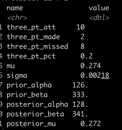
The new player took 10 three point shots, made 2, and has an observed 3pt% of 20%. Using our beta-binomial regression model we estimate the prior for a player with 10 attempts to be 0.274. Combining the prior with the 10 attempts we get a posterior 3pt% for the player of 0.272 (slightly below the average for the population of players who had 10 attempts).

Useful Resources

Some textbooks that I’ve found useful for exploring this type of work:

Deriving a Confidence Interval from an Estimate and a p-value

Although most journals require authors to include confidence intervals into their papers it isn’t mandatory for all journal (merely a recommendation). Additionally, there may be occasions when you are reading an older paper from a time when this mandate/recommendation was not enforced. Finally, sometimes abstracts (due to word count limits) might only present p-values and estimates, in which case you might want to quickly obtain the confidence intervals to help organize your thoughts prior to diving into the paper. In these instances, you might be curious as to how you can get a confidence interval around the observed effect when all you have is a p-value.

Bland & Altman wrote a short piece of deriving confidence interval from only an estimate and a p-value in a 2011 paper in the British Medical Journal:

Altman, DG. Bland, JM. (2011). How to obtain the confidence interval from a p-value. BMJ, 343: 1-2.

Before going through the approach, it is important to note that they indicate a limitation of this approach is that it wont be as accurate in smaller samples, but the method can work well in larger studies (~60 subjects or more).

The Steps

The authors’ list 3 easy steps to derive the confidence interval from an estimate and p-value:

  1. Calculate the test statistic for a normal distribution from the p-value.
  2. Calculate the standard error (ignogre the minus sign).
  3. Calculate the 95% CI using the standard error and a z-critical value for the desired level of confidence.
  4. When doing this approach for a ratio (e.g., Risk Ratio, Odds Ratio, Hazard Ratio), the formulas should be used with the estimate on the log scale (if it already isn’t) and then exponentiate (antilog) the confidence intervals to put the results back to the normal scale.

Calculating the test statistic

To calculate the test statistic use the following formula:

z = -0.862 + sqrt(0.743 – 2.404 * log(p.value))

Calculating the standard error

To calculate the standard error use the following formula (remember that we are ignoring the sign of the estimate):

se = abs(estimate) / z

If we are dealing with a ratio, make sure that you are working on the log scale:

se = abs(log(estimate)) / z

Calculating the 95% Confidence Limits

Once you have the standard error, the 95% Confidence Limits can be calculated by multiplying the standard error by the z-critical value of 1.96:

CL.95 = 1.96 * se

From there, the 95% Confidence Interval can be calculated:

low95 = Estimate – CL.95
high95 = Estimate + CL.95

Remember, if you are working with rate statistics and you want to get the confidence interval on the natural scale, you will need to take the antilog:

low95 = exp(Estimate – CL.95)
high95 = exp(Estimate + CL.95)


Writing a function

To make this simple, I’ll write everything into a function. The function will take three arguments, which you will need to obtain from the paper:

  1. p-value
  2. The estimate (e.g., difference in means, risk ratio, odds ratio, hazard ratio, etc)

The function will default to log = FALSE but if you are working with a rate statistic you can change the argument to log = TRUE to get the results on both the log and natural scales. The function also takes a sig_digits argument, which defaults to 3 but can be changed depending on how many significant digits you need.

estimate_ci_95 <- function(p_value, estimate, log = FALSE, sig_digits = 3){
  
  if(log == FALSE){
    
    z <- -0.862 + sqrt(0.743 - 2.404 * log(p_value))
    z

    se <- abs(estimate) / z
    se
    
    cl <- 1.96 * se
    
    low95 <- estimate - cl
    high95 <- estimate + cl
    
    list('Standard Error' = round(se, sig_digits),
         '95% CL' = round(cl, sig_digits),
         '95% CI' = paste(round(low95, sig_digits), round(high95, sig_digits), sep = ", "))
    
  } else {
    
    if(log == TRUE){
      
      z <- -0.862 + sqrt(0.743 - 2.404 * log(p_value))
      z
      
      se <- abs(estimate) / z
      se
      
      cl <- 1.96 * se
      
      low95_log_scale <- estimate - cl
      high95_log_scale <- estimate + cl
      
      low95_natural_scale <- exp(estimate - cl)
      high95_natural_scale <- exp(estimate + cl)
      
      list('Standard Error (log scale)' = round(se, sig_digits),
           '95% CL (log scale)' = round(cl, sig_digits),
           '95% CL (natural scale)' = round(exp(cl), sig_digits),
           '95% CI (log scale)' = paste(round(low95_log_scale, sig_digits), round(high95_log_scale, sig_digits), sep = ", "),
           '95% CI (natural scale)' = paste(round(low95_natural_scale, sig_digits), round(high95_natural_scale, sig_digits), sep = ", "))
      
    }
    
  }
  
}

 Test the function out

The paper provides two examples, one for a difference in means and the other for risk ratios.

Example 1

Example 1 states:

“the abstract of a report of a randomised trial included the statement that “more patients in the zinc group than in the control group recovered by two days (49% v 32%,P=0.032).” The difference in proportions was Est = 17 percentage points, but what is the 95% confidence interval (CI)?

estimate_ci_95(p_value = 0.032, estimate = 17, log = FALSE, sig_digits = 1)


Example 2

Example 2 states:

“the abstract of a report of a cohort study includes the statement that “In those with a [diastolic blood pressure] reading of 95-99 mm Hg the relative risk was 0.30 (P=0.034).” What is the confidence interval around 0.30?”

Here we change the argument to log = TRUE since this is a ratio statistic needs to be on the log scale.

estimate_ci_95(p_value = 0.034, estimate = log(0.3), log = TRUE, sig_digits = 2)

Try the approach out on a different data set to confirm the confidence intervals are calculated properly

Below, we build a simple logistic regression model for the PimaIndiansDiabetes data set from the {mlbench} package.

  • The odds ratios are already on the log scale so we set the argument log = TRUE to ensure we get results reported back to us on the natural scale, as well.
  • We use the summary() function to obtain the model estimates and p-values.
  • We use the confint() function to get the 95% Confidence Intervals from the model.
  • To get the confidence intervals on the natural scale we also take the exponent, exp(confint()).
  • We use our custom function, estimate_ci_95(), to see how well the results compare.
## get data
library(mlbench)
data("PimaIndiansDiabetes")
df <- PimaIndiansDiabetes

## turn outcome variable into a numeric (0 = negative for diabetes, 1 = positive for diabetes)
df$diabetes_num <- ifelse(df$diabetes == "pos", 1, 0)
head(df)

## simple model
diabetes_glm <- glm(diabetes_num ~ pregnant + glucose + insulin, data = df, family = "binomial")

## model summary
summary(diabetes_glm)


Calculate 95% CI from the p-values and odds ratio estimates.

Pregnant Coefficient

## 95% CI for the pregnant coefficient
estimate_ci_95(p_value = 2.11e-06, estimate = 0.122, log = TRUE, sig_digits = 3)


Glucose Coefficient

## 95% CI for the glucose coefficient
estimate_ci_95(p_value = 2e-16, estimate = 0.0375, log = TRUE, sig_digits = 3)


Insulin Coefficient

## 95% CI for the insulin coefficient
estimate_ci_95(p_value = 0.677, estimate = -0.0003, log = TRUE, sig_digits = 5)


Evaluate the results from the custom function to those calculated with the confint() function.

## Confidence Intervals on the Log Scale
confint(diabetes_glm)

## Confidence Intervals on the Natural Scale
exp(confint(diabetes_glm))

We get nearly the same results with a bit of rounding error!

Hopefully this function will be of use to some people as they read papers or abstracts.

You can find the complete code in a cleaned up markdown file on my GITHUB page.

If the examples we see in textbooks don’t represent the real world, what about the sports science papers we read?

I enjoyed this short article by Andrew Gelman on the blog he keeps with several of his colleagues. The main point, which I agree 100% with, is that the examples in our stats and data analysis textbooks never seem to match what we see in the real world. The examples always seem to work! The data is clean and looks perfectly manicured for the analysis. I get it! The idea is to convey the concept of how different analytical approaches work. The rub is that once you get to the real world and look at your data you end up being like, “Uh. Wait….what is this? What do I do now?!”

The blog got me thinking about something else, though. Something that really frustrates me. If the examples we see in textbooks don’t reflect the data problems we face in the real world, what about the examples we read about in applied sport science research? How much do those examples reflect what we see in the real world?

At the risk of upsetting some colleagues, I’ll go ahead and say it:

I’m not convinced that the research we read in publications completely represents the real world either!

How can that be? This is applied science! Isn’t the real word THE research?

Well, yes and no. Yes, the data was collected in the real world, with real athletes, and in a sport setting. But often, reading a paper, looking at the aim and the conclusions, and then parsing through the methods section to see how they handled the data leaves me scratching my head.

My entire day revolves around looking at data and I can tell you; the real world is very messy.

  • How things get collected
  • How things get saved
  • How things get loaded
  • How things get logged

There are potential hiccups all along the way, no matter how stringent you are in trying to keep sound data collection practices!

In research, the problem is that the data is often touched up in some manner to create an analysis sufficient for publication. Missing values need to be handled a certain way (sometimes those rows get dropped, sometimes values get imputed), class imbalance can be an issue, errant values and outliers from technology flub-ups are a very real thing, data entry issues arise, etc. These things are all problematic and, if not identified prior to analysis, can be a major issue with the findings. I do believe that most people recognize these problems and would agree with me that they are very real issues. However, it is less about knowing that there are problems but rather, figuring out what to do about them. Often the methods sections gloss over these details (I get it, word counts for journals can be a pain in the butt) and simply produce a result that, on paper at least, seems overly optimistic. As I read through the results section, without details about data processing, I frequently say to myself, “No way. There is no way this effect is as real as they report. I can’t reproduce this without knowing how they cleaned up their data to observe this effect.”

Maybe someone should post a paper about how crappy their data is in the applied setting? Maybe we should just be more transparent about the data cleaning processes we go through so that we aren’t overly bullish on our findings and more realistic about the things we can say with confidence in the applied setting?

Does anyone else feel this way? Maybe I’m wrong and I’m being pessimistic, and this isn’t as big of an issue as I believe it to be? Is the data we see in publication truly representative of the real world?

Weakley et al. (2022). Velocity-Based Training: From Theory to Application – R Workbook

Velocity-based training (VBT) is a method employed by strength coaches to prescribe training intensity and volume based off of an individual athlete’s load-velocity profiles. I discussed VBT last year when I used {shiny} to build an interactive web application for visualizing and comparing athlete outputs.

Specific to this topic, I recently read the following publication: Weakley, Mann, Banyard, McLaren, Scott, and Garcia-Ramos. (2022). Velocity-based training: From theory to application. Strength Cond J; 43(2): 31-49.

The paper aimed to provide some solutions for analyzing, visualizing, and presenting feedback around training prescription and performance improvement when using VBT. I enjoyed the paper and decided to write an R Markdown file to provide code that can accompany it and (hopefully) assist strength coaches in applying some of the concepts in practice. I’ll summarize some notes and thoughts below, but if you’d like to read the full R Markdown file that explains and codes all of the approaches in the paper, CLICK HERE>> Weakley–2021—-Velocity-Based-Training—From-Theory-to-Application—Strength-Cond-J.

If you’d like the CODE and DATA to run the analysis yourself, they are available on my GitHub page.

Paper/R Markdown Overview

Technical Note: I don’t have the actual data from the paper. Therefore, I took a screen shot of Figure 3 in the text and used an open source web application for extracting data from figures in research papers. This requires me to go through and manually click on the points of the plot itself. Consequently, I’m not 100% perfect, so there may be subtle differences in my data set compared to what was used for the paper.

The data used in the paper reflect 17-weeks of mean concentric velocity (MCV) in the 100-kg back squat for a competitive powerlifter, tested once a week. The two main figures, which, along with the analysis, I will recreate are Figure 3 and Figure 5.

Figure 3 is a time series visual of the athlete while Figure 5 provides an analysis and visual for the athlete’s change across the weeks in the training phase.

Figure 3

The first 10-weeks represent the maintenance phase for the athlete, which was followed by a 7-week training phase. The maintenance phase sessions were used to build a linear regression model which was then used to visualize the athlete’s change over time along with corresponding confidence interval around each MCV observation. The model output looks like this:

The standard (typical) error was used to calculate confidence intervals around the observations. To calculate the standard error, the authors’ recommend one of two approaches:

1) If you have group-based test-retest data, they recommend taking the difference between the test-retest outcomes and calculating the standard error as follows:

  • SE.group = sd(differences) / sqrt(2)

2) If you have individual observations, they recommend calculating the standard error like this:

  • SE.individual = sqrt(sum.squared.residuals) / (n2))

Since we have individual athlete data, we will use the second option, along with the t-critical value for 80% CI, to produce Figure 3 from the paper :

The plot provides a nice visual of the athlete over time. We see that, because the linear model is calculated for the maintenance phase, as time goes on, the shaded standard error region gets wider. The confidence intervals around each point estimate are there to encourage us to think past just a point estimate and recognize that there is some uncertainty in every test outcome that cannot be captured in a single value.

Figure 5

This figure visualizes the change in squat velocity for the powerlifter in weeks 11-17 (the training phase) relative to the mean squat velocity form the maintenance phase, representing the athlete’s baseline performance.

Producing this plot requires five pieces of information:

  1. Baseline average for the maintenance phase
  2. The difference between the observed MVC in each training week and the maintenance average
  3. Calculate the t-critical value for the 90% CI
  4. Calculate the Lower 90% CI
  5. Calculate the Upper 90% CI

Obtaining this information allows us to produce the following table of results and figure:

Are the changes meaningful?

One thing the authors’ mention in the paper are some approaches to evaluating whether the observed changes are meaningful. They recommend using either equivalence tests or second generation p-values. However, they don’t go into calculating such things on their data. I honestly am not familiar with the latter option, so I’ll instead create an example of using an equivalence test for the data and show how we can color the points within the plot to represent their meaningfulness.

Equivalence testing has been discussed by Daniel Lakens and colleagues in their tutorial paper, Lakens, D., Scheel, AM., Isager, PM. (2018). Equivalence testing for psychological reserach: A tutorial. Advances in Methods and Practices in Psychological Science. 2018; 1(2): 259-269.

Briefly, equivalence testing uses one-sided t-tests to evaluate whether the observed effect is larger or smaller than a pre-specified range of values surrounding the effect of interest, termed the smallest effect size of interest (SESOI).

In our above plot, we can consider the shaded range of values around 0 (-0.03 to 0.03, NOTE: The value 0.03 was provided in the text as the meaningful change for this athlete to see an ~1% increase in his 1-RM max) as the region where an observed effect would not be deemed interesting. Outside of those ranges is a change in performance that we would be most interested in. In addition to being outside of the SESOI region, the observed effect should be substantially large enough relative to the standard error around each point, which we calculated from our regression model earlier.

Putting all of this together, we obtain a the same figure above but now with the points colored specific to the p-value provided from our equivalence test:

Warpping Up

Again, if you’d like the full markdown file with code (click the ‘code’ button to display each code chunk) CLICK HERE >> Weakley–2021—-Velocity-Based-Training—From-Theory-to-Application—Strength-Cond-J

There are always a number of ways that analysis can unfold and provide valuable insights and this paper reflects just one approach. As with most things, I’m left with more questions than answers.

For example, Figure 3, I’m not sure if linear regression is the best approach. As we can see, the grey shaded region increases in width overtime because time is on the x-axis (independent variable) and the model was built on a small portion (the first 10-weeks) of the data. As such, with every subsequent week, uncertainty gets larger. How long would one continue to use the baseline model? At some point, the grey shaded region would be so wide that it would probably be useless. Are we too believe that the baseline model is truly representative of the athlete’s baseline? What if the baseline phase contained some amount of trend — how would the model then be used to quantify whatever takes place in the training phase? Maybe training isn’t linear? Maybe there is other conditional information that could be used?

In Figure 5, I wonder about the equivalence testing used in this single observation approach. I’ve generally thought of equivalence testing as a method comparing groups to determine if the effect from an intervention in one group is larger or smaller than the SESOI. Can it really work in an example like this, for an individual? I’m not sure. I need to think about it a bit. Maybe there is a different way such an analysis could be conceptualized? A lot of these issues come back to the problem of defining the baseline or some group of comparative observations that we are checking our most recent observation against.

My ponderings aside, I enjoyed the paper and the attempt to provide practitioners with some methods for delivering feedback when using VBT.

Issues with ‘Black Box’ Machine Learning Models in Injury Prediction

Injury prediction models developed using machine learning approaches have become more common due to the substantial rise of proprietary software in the sports science and sports medicine space. However, such ‘black box’ approaches are not without limitation. Aside from a lack of transparency, preventing independent evaluation of model performance, these types of models present challenges in interpretation, making it difficult for practitioners who are required to make decisions about athlete health and plan interventions.

I recently had the pleasure of working on a paper headed up by Garrett Bullock and a list of wonderful co-authors where we discuss some of these issues:

Black Box Prediction Methods in Sports Medicine Deserve a Red Card for Reckless Practice: A Change of Tactics is Needed to Advance Athlete Care. Sports Med.