Category Archives: Model Building in Python

Comparing Tidymodels in R to Scikit Learn in Python

I did a previous blog providing a side-by-side comparisons of R’s {tidyverse} to Python for various data manipulation techniques. I’ve also talked extensively about using {tidymodels} for model fitting (see HERE and HERE). Today, we will work through a tutorial on how to fit the same random forest model in {tidyverse} and Scikit Learn.

This will be a side-by-side view of both coding languages.The tutorial will cover:

  • Loading the data
  • Basic exploratory data analysis
  • Creating a train/test split
  • Hyperparameter tuning by creating cross-validated folds on the training data
  • Identifying the optimal hyperparameters and fitting the final model
  • Applying the final model to the test data and evaluating model performance
  • Saving the model for downstream use
  • Loading the saved model and applying it to new data

To get the full code for each language and follow along with the tutorial visit my GITHUB page.
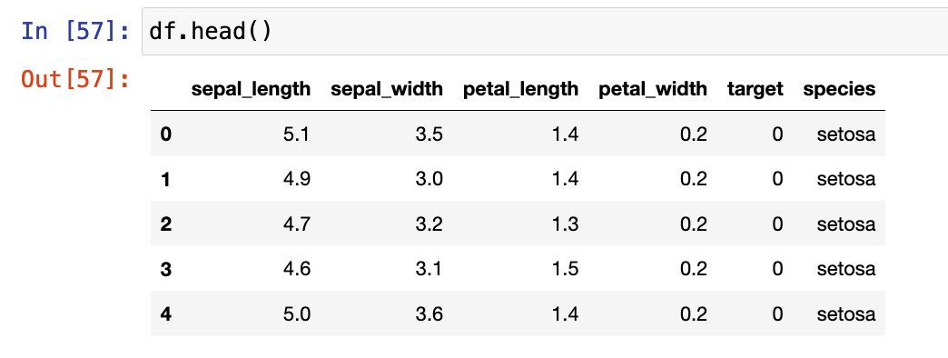
The Data

The data comes the tidytuesday project from 4/4/2023. The data set is Premier League match data (2021 – 2022) that provides a series of features with the goal of predicting the final result (Full Time Result, FTR) as to whether the home team won, the away team won, or the match resulted in a draw.

Load Data & Packages

First, we load the data directly from the tidytuesday website in both languages.

Exploratory Data Analysis

Next, we perform some exploratory data analysis to understand the potential features for our model.

  • Check each column for NAs
  • Plot a count of the outcome variable across the three levels (H = home team wins, A = away team wins, D = draw)
  • Select a few features for our model and then create box plots for each feature relative to the 3 levels of our outcome variable

Train/Test Split

We being the model building process by creating a train/test split of the data.

Create a Random Forest Classifier Instance

This is basically telling R and python that we want to build a random forest classifier. In {tidymodels} this is referred to as “specifying the model engine”.

Hyperparameter Tuning on Cross Validated Folds

The two random forest hyperparameters we will tune are:

  1. The number of variables randomly selected for candidate model at each split (R calls this mtry while Python calls it max_features)
  2. The number of trees to grow (R calls this trees and Python calls it n_estimators)

In {tidymodels} we will specify 5 cross validated folds on the training set, set up a recipe, which explains the model we want (predicting FTR from all of the other variables in the data), put all of this into a single workflow and then set up our tuning parameter grid.

In Scikit Learn, we set up a dictionary of parameters (NOTE: they must be stored in list format) and we will pass them into a cross validation structure that performs 5-fold cross-validation in parallel (to speed up the process). We then pass this into the GridSearchCV() function where we specify the model we are fitting (random forest), the parameter grid that we’ve specified, and how we want to compare the random forest models (scoring). Additionally, we’ll set n_jobs = -1 to allow Python to use all of the cores on our machine.

While the code looks different, we’ve essentially set up the same process in both languages.

Tune the model on the training data

We can now tune the hyperparameters by applying the cross-validated folds procedure to the training data.

Above, we indicated to Python that we wanted some parallel processing, to speed up the process. In {tidyverse} we specify parallel processing by setting up the number of cores we’d like to use on our machine. Additionally, we will want to save the results of each cross-validated iteration, so we use the control_sample() function to do this. All of these steps were specified in Python, above, so we are ready to now apply cross-validation to our training dataset and tune the hyperparameters.

Get the best parameters

Both R and Python provide numerous objects to explore the output for each of the cross-validated folds. I’ve placed some examples in the respective codes in the GITHUB page. For our purposes, we are most interested in the optimal number of variables and trees. Both coding languages found 4 and 400 to be the optimal number of variables and trees, respectively.

Fitting the Final Model

Now that we have the optimal hyperparameter values, we can refit the model. In both {tidymodels} and Scikit learn, we’ll just refit a random forest with those optimal values specified.

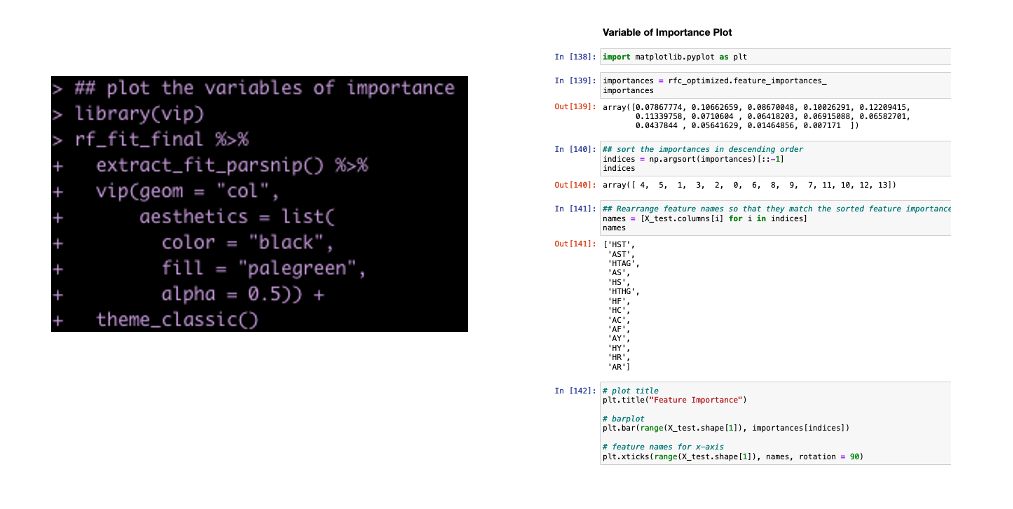
Variable Importance Plot

It’s helpful to see which variables were the most important contributors to the model’s predictions.

Side Note: This takes more code in python than in R. This is one of the drawbacks I’ve found with python compared to R. I can do things more efficiently and with less code in R than in python. I often find I have to work a lot harder in Scikit Learn to get model outputs and information about the model fit. It’s all in there but it is not clearly accessible (to me at least) and plotting in matplotlib is not as clean as plotting in ggplot2.

Get Model Predictions on the Test Set

Both languages offer some out of the box options for describing the model fit info. If you want more than this (which you should, because this isn’t much to go off of), then you’ll have to extract the predicted probabilities and the actual outcomes and code some additional analysis (potentially a future blog article).

Save The Model

If we want to use this model for any downstream analysis we will need to save it.

Load the Model and Make Predictions

Once we have the model saved we can load it and apply it to any new data that comes in. Here, our new data will just be a selection of rows from the original data set (we will pretend it is new).

NOTE: Python is 0 indexed while R is indexed starting at 1. So keep that in mind if selecting rows from the original data to make the same comparison in both languages.

Wrapping Up

Both {tidymodels} and Scikit Learn provide users with powerful machine learning frameworks for conducting analysis. While the code syntax differs, the general concepts are the same, so bouncing between the two languages shouldn’t be to cumbersome. Hopefully this tutorial provided a nice overview of how to conduct the same analysis in both languages, offering a bridge for those trying to learn Python from R and vice versa.

All code is available on my GITHUB page.

Bayesian Linear Regression: Getting started with PyMC3

Previously I’ve used {rstanarm}, {brms}, and Stan for fitting Bayesian models. However, as I continue to work on improving my Python skills, I figured I’d try and delve into the PyMC3 framework for fitting such models. This article will go through the following steps:

  1. Fitting the model
  2. Making a point estimate prediction
  3. Making a point estimate prediction with uncertainty
  4. Calculating a posterior predictive distribution

I’ve covered the last three steps in a prior blog on making predictions with a Bayesian model. I know there are probably functions available in PyMC3 that can do these things automatically (just as there are in {rstanarm}) but instead of falling back on those, I create the posterior distributions here using numpy and build them myself.

The entire code and data are available on my GITHUB page, where I also have the model coded in {rstanarm}, for anyone interested in seeing the steps in a different code language.

Loading Libraries & Data

The data I’ll be using is the {mtcars} data set, which is available in R. I’ve saved a copy in .csv format so that I can load it into my Jupyter notebook.

import pandas as pd
import numpy as np
import matplotlib.pyplot as plt 
import seaborn as sns
import pymc3 as pm
import arviz as az 
import os

# load mtcars
d = pd.read_csv('mtcars.csv')
d.head()

Exploratory Data Analysis

The model will regress mpg on engine weight (wt). Let’s plot and describe those two variables so that we have a sense for what we might be working with.

Linear Regression

Before fitting the Bayesian model, I want to fit a simple regression model to see what the coefficients look like.

import statsmodels.api as sm

x = d['wt']
y = d['mpg']

x = sm.add_constant(x)

fit = sm.OLS(y, x).fit()

fit.summary()

We can see that for every one unit increase in engine weight the miles per gallon decrease, on average, by about 5.3.

Bayesian Regression (PyMC3)

Fitting a Bayesian regression model in PyMC3 requires us to specify some priors. For this model I’ll use a prior intercept of 40 ± 10 and a prior beta for the wt variable of 0 ± 10. The thing to note here is that the priors I’m specifying priors were created by first looking at the data that has been collected (which is technically cheating). Normally we would have priors BEFORE collecting our data (using prior published research, data from a pilot study, prior intuition, etc) and then combine the prior with the observations to obtain a posterior distribution. However, the aim here is to understand how to code the model, so I’ll use these priors. I’ll write a longer blog on priors and what they do to a model in the coming weeks.

Some notes on fitting the model in PyMC3:

  • The model is named ‘fit_b
  • We specify the intercept as variable ‘a
  • The beta coefficient for wt is called ‘b
  • Both the intercept and slope re fit with normally distributed priors
  • Finally, ‘e‘ represents the model error and it is fit with a a Half Cauchy prior
  • Once the priors are set, the model is specified (y_pred) as mu = a + b * wt + e
  • The trace_b object stores our posterior samples, 2000 of them of which the first 1000 will be discarded because they are there to allow the model to tune itself
, sd = e, observed = d['mpg'])
    
    trace_b = pm.sample(2000, tune = 1000)


Once the model has been fit we plot the trace plots to see how well it performed.

We can also directly call the mean and standard deviation values of our fitted model, which are relatively similar to what we saw with the linear regression model above.

Point Predictions

Next, we want to make a single point prediction for the mpg would expect, on average, when wt  is a specific value (in this example we will use wt = 3.3).

To do this, we simply store the average value of the posterior coefficients from our Bayesian regression and apply the specified model:

mu = a + b * new_wt

A car with an engine weight of 3.3 would get, on average, 19.7 mpg.

Point Prediction with Uncertainty

The point estimate is interesting (I guess), but there is uncertainty around that estimate as point predictions are never exact. We can compliment this point estimate by unveiling the uncertainty around it. The point prediction ± uncertainty interval informs us of the average value of  mpg along with the uncertainty of the coefficients in our model.

To do this, we create a random sample of 1000 values from the posterior distributions for our model intercept and beta coefficient. Each of these 1000 values represent a potential intercept and slope that would be consistent with our data, which shows us the uncertainty that we have in our estimates. When we use the model equation, multiplying each of these 1000 values by the new_wt value we obtain 1000 possible predicted values of mpg given a weight of 3.3.

With this posterior distribution we can then plot a histogram of the results and obtain summary statistics such as the mean, standard deviation, and 90% credible interval.

Posterior Predictive Distribution

Finally, instead of just knowing the average predicted value of mpg ± uncertainty for the population, we might be interested in knowing what the predicted value of mpg would be for a new car in the population with a wt of 3.3. For that, we calculate the posterior predictive distribution. The uncertainty in this predictive distribution will be larger than the point prediction with uncertainty because we are using the posterior model error added to our prediction.

First, similar to the model coefficients, we have to get the random draws of our error term, which we will call sigma.

Next, we run the model as we did in step 2 above; however, we also add to each of the 1000 posterior predictions the sigma value by taking a random draw from a normal distribution with a mean of 0 and standard deviation equal to the sigma sample values.

pred_dist = intercept_sample + beta_sample * new_wt_rep + np.random.normal(loc = 0, scale = sigma_sample, size = 1000)


Finally, we plot the distribution of our predicted values along with the mean, standard deviation, and 90% credible interval. Notice that these values are larger than what we obtained in step 2 because we are now taking into account additional uncertainty about the new wt observation.

Wrapping Up

That’s a brief intro to Bayesian regression with PyMC3. There are a lot more things that we can do with PyMC3 and it’s available functions. My goal is to put together more blog articles on Bayesian modeling with both R and Python so show their flexibility. If you spot any errors, please let me know.

The data and full code (along with a companion code in {rstanarm}) is available on my GITHUB page.

t-test…ANOVA…It’s linear regression all the way down!

I had someone ask me a question the other day about t-tests. The question was regarding how to get the residuals from a t-test. The thing we need to remember about t-tests and ANOVA is that they are general linear models. As such, an easier way of thinking about them is that they are a different way of looking at a regression output. In this sense, a t-test is just a simple linear regression with a single categorical predictor (independent) variable  that has two levels (e.g., Male & Female) while ANOVA is a simple linear regression with a single predictor variable that has more than two levels (e.g., Cat, Dog, Fish).

Let’s look at an example!

Complete code is available on my GITHUB page.

Load Data

The data we will use is the iris data set, available in the numpy library.

Exploratory Data Analysis

The Jupyter Notebook I’ve made available on GITHUB has a number of EDA steps. For this tutorial the variable we will look at is Sepal Length, which appears to different between Species.

T-test

We will start by conducting a t-test. Since a t-test is a comparison of means between two groups, I’ll create a data set with only the setosa and versicolor species.

## get two groups to compare
two_groups = ["setosa", 'versicolor']

## create a data frame of the two groups
df2 = df[df['species'].isin(two_groups)]

First I build the t-test in two common stats libraries in python, statsmodels and scipy.

## t-test in statsmodels.api
smf.stats.ttest_ind(x1 = df2[df['species'] == 'setosa']['sepal_length'],
                    x2 = df2[df['species'] == 'versicolor']['sepal_length'],
                   alternative="two-sided")

## t-test in scipy
stats.ttest_ind(a = df2[df['species'] == 'setosa']['sepal_length'],
                b = df2[df['species'] == 'versicolor']['sepal_length'],
                alternative="two-sided")

Unfortunately, the output of both of these approaches leaves a lot to be desired. They simply return the t-statistics, p-value, and degrees of freedom.

To get a better look at the underlying comparison, I’ll instead fit the t-test using the researchpy library.

## t-test in reserachpy
rp.ttest(group1 = df2[df['species'] == 'setosa']['sepal_length'],
         group2 = df2[df['species'] == 'versicolor']['sepal_length'])

This output is more informative. We can see the summary stats for both groups at the top. the t-test results follow below. We see the observed difference, versicolor has a sepal length 0.93 (5.006 – 5.936) longer that setosa, on average. We also get the degrees of freedom, t-statistic, and p-value, along with several measures of effect size.

Linear Regression

Now that we see what the output looks like, let’s confirm that this is indeed just linear regression!

We fit our model using the statsmodels library.

## Linear model to compare results with t-test (convert the species types of dummy variables)
X = df2[['species']]
X = pd.get_dummies(X['species'], drop_first = True)

y = df2[['sepal_length']]

## add an intercept constant, since it isn't done automatically
X = smf.add_constant(X)

# Build regression model
fit_lm = smf.OLS(y, X).fit()

# Get model output

fit_lm.summary()

Notice that the slope coefficient for versicolor is 0.93, indicating it’s sepal length is, on average, 0.93 greater than setosa’s sepal length. This is the same result we obtained with our t-test above.

The intercept coefficient is 5.006, which means that when versicolor is set to “0” in the model (0 * 0.93 = 0) all we are left with is the intercept, which is the mean value for setosa’s sepal length, the same as we saw in our t-test.

What about the residuals?

The question original question was about residuals from the t-test. Recall, the residuals are the difference between actual/observed value and the predicted value. When we have a simple linear regression with two levels (a t-test) the predicted value is simply the overall mean value for that group.

We can add predictions from the linear regression model into our data set and calculate the residuals, plot the residuals, and then calculate the mean squared error.

## Add the predictions back to the data set
df2['preds'] = fit_lm.predict(X)

## Calculate the residual
resid = df2['sepal_length'] - df2['preds']

## plot the residuals
sns.kdeplot(resid,shade = True)
plt.axvline(x = 0,linewidth=4, linestyle = '--', color='r')

In the code, you will find the same approach taken by just applying the group mean as the “predicted” value, which is the same value that the model predicts. At the bottom of the code, we will find that the outcome of the MSE is the same.

Wrapping Up

In summary, whenever you think t-test or ANOVA, just think linear regression. The intercept will end up reflecting the mean value for the reference class while the coefficient(s) for the other classes of that variable will represent the difference between their mean value and the reference class. If you want to make a comparison to a different reference class, you can change the reference class before specifying your model and you will obtain a different set of coefficients (given that they are compared to a new reference class) but the predicted values, residuals, and MSE will end up being the same.

Again, if you’d like the full code, you can access it HERE.

Python Tips & Tricks: Coding A Tensorflow Neural Network to Predict Yards After Catch

As I work to improve my python skills, I’ll keep adding my efforts to the blog. This week, I saw a nice article showing a basic approach to coding a neural network in R to predict yards after catch in NFL receivers from the folks at www.opensourcefootball.com. So, I decided to take that idea and try and create my own neural network in Python.

Some notes:

  1. This is not a to say that the neural network was the best method to answer the question. Rather, it was just a way for me to try and take stuff I’d already do in R and see if I could learn it in Python.
  2. This is not a blog post to cover all aspects of neural networks (not even close). It just so happened that the original article used a neural network via tensorflow in R and I happened to be doing some work in tensorflow in Python this week, so it was an easy connection to make.
  3. My Python coding is pretty messey and at times I feel like it takes me several steps to do what someone might do in a few lines. Feel free to comment and offer suggestions.
  4. Harking back to point one, I finish the script by coding a linear regression model to answer the same question (predict yards after catch) as it is a simpler and more interpretable than a neural network. I construct the regression model in two ways. First, I do it in sklearn, which seems to be the preferred approach to coding models by pythoners. I then do it in the statsmodels library. I’m sure this is more a function of my poor python programming skills but I do feel like the model output from statsmodels is more informative than what I can get returned from sklearn (and I show this in the script).

The data came from nflfastR, which is an R package for obtaining NFL play-by-play data created by Ben Baldwin et al.

I provide a step-by-step explanation for coding the model on my GITHUB page.


Python Tips & Tricks: Random Forest Classifier for TidyX Episode 18

As a means of working on improving some of my Python skills, I decided I’ll attempt to re-create different elements from some of our TidyX Screen Casts.

This past week, we did an episode on building a random forest classifier for coffee ratings (CLICK HERE). I’ve recreated almost all of the steps that we did in R in Python Code.

1) Loading the data from the TidyTuesday github page.

2) Data pre-processing

3) Exploratory data analysis

4) Random Forest classifier development and model testing


You can access the full Jupyter Notebook on my GITHUB page. I’m still trying to get the hang of Python so if there are any Pythonistas out there that have feedback or see errors in my code, I’m all ears!