This week I was listening to Layne Norton’s Podcast Interview with Bill Campbell on training and nutrition research. I found it to be an interesting listen. Layne has been in this space for a long time (he and I started out on the same internet forum back in the early 2000’s, Avant Labs — RIP Patrick Arnold). Layne always does a nice job at trying to combat a lot of the nonsense that takes place in the health and fitness space (with internet influencers pedaling whatever the latest supplement or training program is). I also have enjoyed much of the work that Bill Campbell has put out (we even published a paper together many years ago).
In this podcast, the two get into a discussion about protein intake and Bill makes the statement that you can overeat your calories and as long as the surplus is coming from protein the evidence seems to suggest that you’d be hard pressed to put on excess body fat and, in fact, gain some muscle. Layne is skeptical of this and the two discuss a few potential hypotheses of why this may be, ultimately concluding that Layne would do a bit of a deep dive into the literature — I’ll be interested to see what he finds.
During the discussion, Bill referenced one of his papers, Effects of high vs. low protein intake on body composition and maximal strength in aspiring female physique athletes engaging in an 8-week resistance training program. I decided to pull the paper and give it a read. In the process of reading it, I decided to pull out my laptop and write a simulation of aspects of the study (primarily calories and fat free mass) to better understand the results, explore uncertainty (it was only 17 subjects) and create a slightly different model (Bayesian hierarchical model) to show how we can understand more about where the variance is coming from and what we can learn from that.
I wont hash out al of the code here. If you want the full coded simulation you can download it from my GITHUB page and knit it from there if you want to also see it in an HTML form.
With that said, let’s dive in…
Introduction
- Individuals participating in a regimented resistance training program require more protein than that of sedentary individuals. Recent research has suggested that requirements may be as high as 2.2 g/kg/day (1g/lb/day) in a young bodybuilder population.
- However, longitudinal studies are lacking and many of the studies conducted up to this point have some methodological flaws (e.g., unsupervised training programs). Additionally, there is a paucity of such research in female populations.
Study Aim: The purpose of this study was to investigate the effects of higher versus lower daily protein intakes on body composition changes in aspiring female physique athletes following a supervised daily undulating periodized resistance training program.
Conclusions up front
NOTE: If you don’t want to read the nitty-gritty down below the primary take away from the study is on protein, calories, and increases in lean mass and decreases in fat mass:
- A high-protein diet of 2.4 grams protein/kg/day (1.1g/lb/day) increased Fat Free Mass compared to a low-protein diet of 1.2 grams protein/kg/day (0.5g/lb/day)
- These findings are similar to those of prior studies — though many of these studies have limitations such as the duration of time the study can be run, the population studied, the inability to control other aspects of diet or sometimes training, and the issue with sample size (most higher level trainees are not looking to be a part of a study where they could potentially end up in a control group and be forced to train and eat sub-optimally for 8-12 weeks)
- Importantly, the high-protein group also saw increased calorie intake compared to the low-protein group. Despite this, they still lost more body fat and gained more muscle mass. So, calories went up (with the excess of calories coming from protein) and body composition results improved!! It was hypothesized that this may be due to the increased calories from additional protein being used to help build lean tissue (as opposed to being stored as adipose tissue) and the higher levels of protein potentially having a positive influence on the energy expenditure side of the energy balance equation.
Goal of this simulation
- The aim of this simulation is to try and recreate some of the analysis and better understand the observed data from the 17 participants.
- The goal of this simulation is not to say that the study is wrong or incorrect or point out flaws. Generally, I am in favor of high protein diets (I’m a meathead at heart) and the results from this study are part of a bigger body of literature on protein intake, which despite study limitations (every study has some) generally seems to favor higher levels of protein for those with strength and physique based goals.
Methods
Design
- Parallel group, repeated measures design
- Subjects were randomized to a high protein or low protein diet group in conjunction with a supervised resistance training program for 8-weeks
- Participants were healthy aspiring female physique athletes who were required to have been resistance training for the prior three months or longer and needed to be able to deadlift 1.5x body weight
Diet Groups
- High Protein Group (n = 8) = 2.4 grams protein/kg/day (1.1g/lb/day)
- Low Protein Group (n = 9) = 1.2 grams protein/kg/day (0.5g/lb/day)
- NOTE: Subjects tracked all food intake but no restrictions were placed on dietary carbohydrate or fat intake.
Workouts
- 8-week training program (28 sessions)
- 2 upper body and 2 lower body sessions per week
- Lower body consisted of 5 exercises per session
- Upper body consisted of 6 exercises per session
- Sets and reps varied throughout the program and included ranges such as 3-5 reps, 9-11 reps, 14-16 reps
- Subjects self-selected loads that would allow them to complete the appropriate number of reps within the specified rep range allowing for one rep in reserve
- Subjects also performed a high intensity interval program consisting of 30-sec sprints with 2min of rest between sets using their modality of choice (treadmill, sprinting, cycle ergometer, rowing machine, etc)
Statistics
- Dependent Variables
- Body Comp (fat-free mass, fat mass, body fat%)
- Max strength (back squat and deadlift)
- Resting metabolic rate
- Nutrition intake data was analyzed with independent sample t-tests
- Data for the dependent variables were analyzed with a 2-group (high vs moderate protein) * 2-time point (pre- and post-training) between-within factorial ANOVA with repeated measures
Results
- This result section leaves a lot to be desired. It is literally a paragraph of about 30 words that basically say, “see the tables”. The authors then talk about the results in the discussion section as they pertain to prior research. However, the discussion section should be for the researchers to talk about their interpretation of the research (what they found, why they think the results were the way they were, how the results compare with other studies, what potential research should be done in the future to better understand the phenomenon, limitations of the study, etc). So, we don’t have a clear explanation of the observed data in the results section.
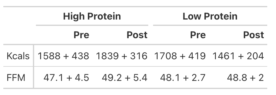
- To try and better understand the data, we will recreate the analysis for Kcals (Table 1) and then build a simulation to better understand the analysis for Fat Free Mass (Table 2).
KCals
- Kcals were analyzed with an independent t-test
- Table 1 of the paper provides the pre- and post-mean Kcals for both groups and indicates a statistically significant effect.
- We can easily calculate the change score for both groups (the change from pre to post). But, to calculate the standard deviation of the change score, which we need when conducting an independent t-test, we need to use a little bit of math to help us. We will estimate the standard deviation of the change scores for both groups using the pre- and post-test standard deviations provided in the table and then take a guess that the correlation between pre- and post-tests is relatively high, say, `r = 0.85`.
We will investigate the Kcals in two different ways:
- Calculate a t-test by hand
- Calculate a Cohen’s D Effect Size Statistic to help us understand the magnitude of the effect
T-test

Cohen’s D Effect Size
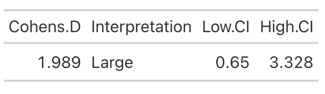
- From the t-test we conclude that the high protein group consumed, on average, 498 more Kcals (+/- 121.3) than the low protein group. It’s important to note that most of these extra calories came from protein and, although the high protein group increased their calories they actually lost body fat and increased muscle mass (as we will see below) relative to the low protein group!
- Cohen’s D tells us that the magnitude of the effect ranges from medium to large, indicating that the high protein group saw a rather large increase in calories relative to the low protein group
Analyzing Fat Free Mass
- This is where things get interesting. We need the actual raw data to run a between-within factorial ANOVA with repeated measures. Soooo…that means we will have to simulate the study (since we don’t have raw data), which is tricky because we don’t know enough about the sources of variance between and within the groups. So, we will need to make some assumptions.
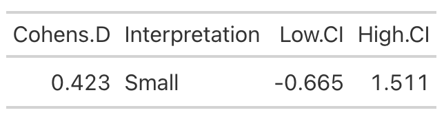
- Looking at Fat-Free Mass from Table 2, we see that the author’s produced a Cohen’s d effect size for the change in fat-free mass from pre- to post-testing for both the high- and low-protein groups. Let’s first calculate those using the function we built above.
High Protein Group Effect Size
Low Protein Group Effect Size
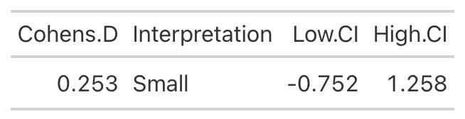
- Using the data from Table 2 of the paper, we easily re-create the point estimate for Cohen’s d. The authors did not produce the confidence interval around the effect statistic, but that shouldn’t stop us! We can see from our outputs above, in both cases the 95% Confidence Interval around the observed Cohen’s d ranges from negative to positive. This indicates that, while the author’s did find a statistically significant effect for the change in Fat-Free Mass, there is some uncertainty around the magnitude of this change. The high-protein group did have a standard deviation that was nearly 2x larger than that observed for the low-protein group. So, we don’t really know how the individuals in the high-protein group looked. Perhaps a few of them saw a really large effect, a few of them saw an effect more similar to that of the low-protein group, and a few of them saw a worse effect? We simply don’t know with the data being presented as it is. A change looks like it took place but their analysis doesn’t allow us to tease out the within-subject variability. Perhaps some people saw better results (for any number of reasons) than others. We’d love to know this!
Simulating the Fat Free Mass variable
- We will turn to simulation to get a grasp of what might be taking place in this study. We know that the author’s find a statistically significant effect, but we want to try and put into perspective how certain we should be (after-all, it is only 17 subjects).
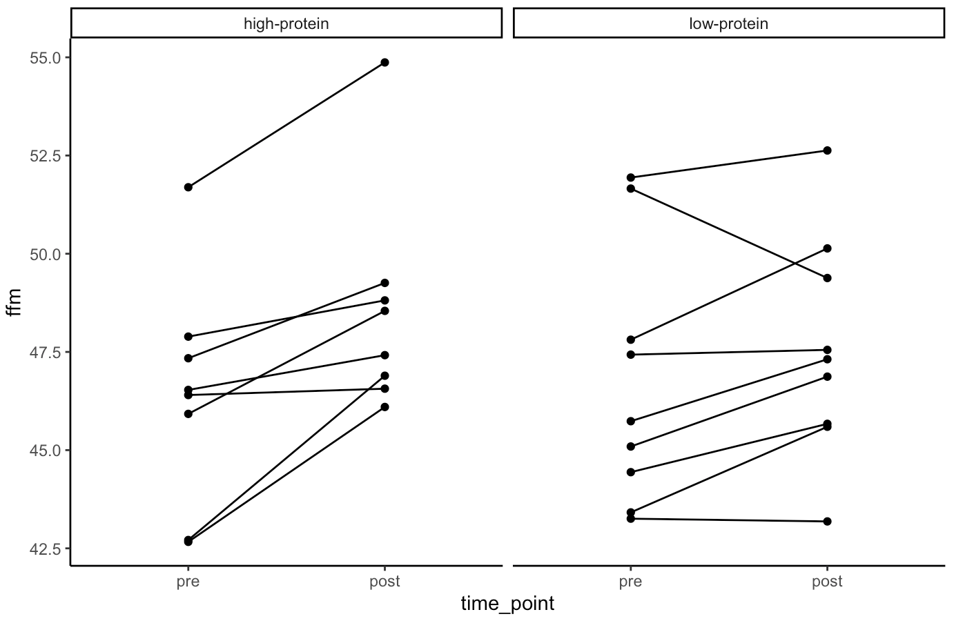
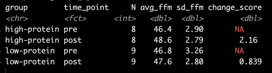
- Our simulation looks similar to the results presented in the study for FFM. We see that the high-protein group increased their FFM be 2.2kg, on average, while the low-protein group only increased by 0.85 kg, on average.
- From the plots we can see thas that in the simulated data, a few of the subjects in the high-protein group had very dramatic increases in FFM, while some of the others saw smaller improvements and one appeared to stay the same. The simulated low-protein group shows two of the subjects actually decreased their FFM. one stayed relatively the same, and the others saw small increases in FFM.
Model
- Next, we take our simulated data set and we construct a model. The authors used a between-within factorial ANOVA with repeated measures. Instead, of doing this, I’m going to build a hierarchical mixed model so that we can better explore the the sources of variance in the data. We will use a Bayesian hierarchical model so that we can get the full posterior distribution. Our fixed effects will be group, time, and a group*time interaction and our random effects will consisted of a random intercept slope across time points for each subject.
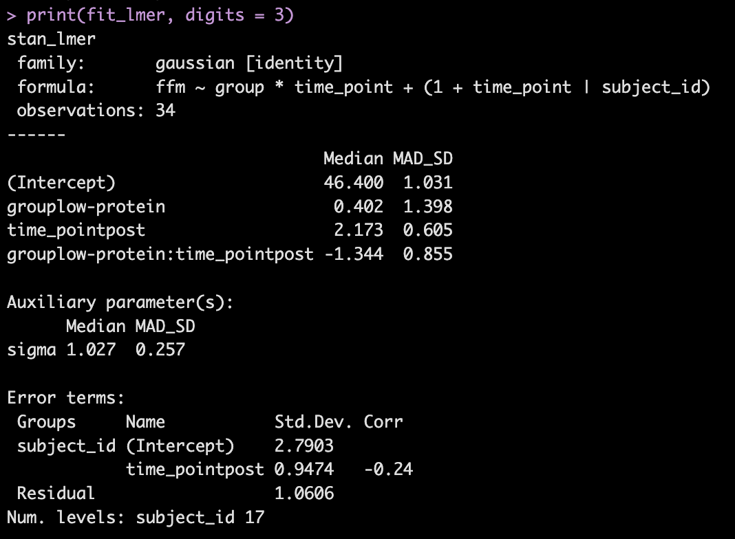
- The model recovers the parameters that we used for our simulation (the ground truth) as it should, as this is how we built the model.
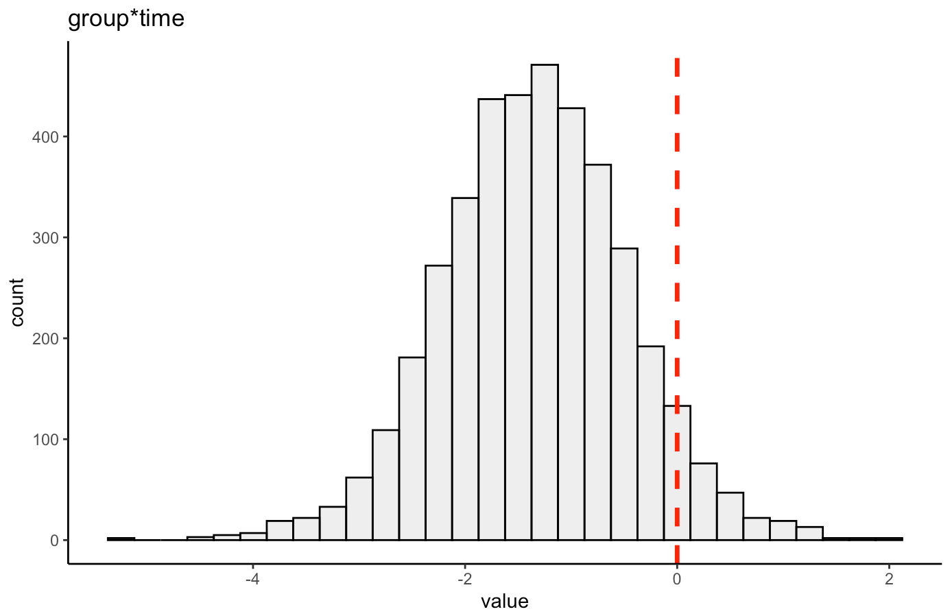
- The group*time interaction indicates the difference in the slope (change) between the two groups from pre to post. Here, -1.3 indicates that the low protein group experienced 1.3kg less improvement in FFM than the high-protein group.
- In Table 2 we see that the high-protein group increased FFM, on average, by 2.0kg and the low-protein group by 0.6kg, on average, which is a -1.4kg difference between the groups (`0.6 – 2.0 = -1.4`), which is very closer to our interaction of -1.3
We can get credible intervals for the mixed effects from the model
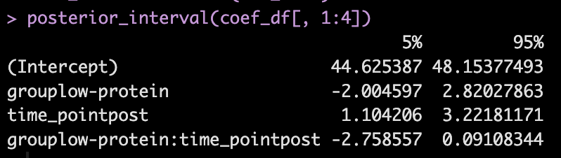
- Here, the 90% credible interval for the group*time interaction ranges from -2.7 to 0.09. So, we have a rather wide range of uncertainty in the credible interval, where it may be plausible that there is no difference in the two groups during the post-test FFM. There is 90% confidence that the change in FFM differs between the low and high group from -2.8 kg to nearly a 0.1 kg increase in FFM for the low-protein group (compared to the high protein group).
We can also plot the posterior distribution for the group*time interaction
Random Effects
- From our model output, the random effects (Error Terms) tell is that the between subject standard deviation is 2.8 and the within subject standard deviation (Residual) is 1.1. We also see that the random effect for the time_point slope is 0.95.
- We can get a table of the regression equation for each subject, incorporating their random intercept and slopes (notice how Intercept and time_pointpost differ for each)
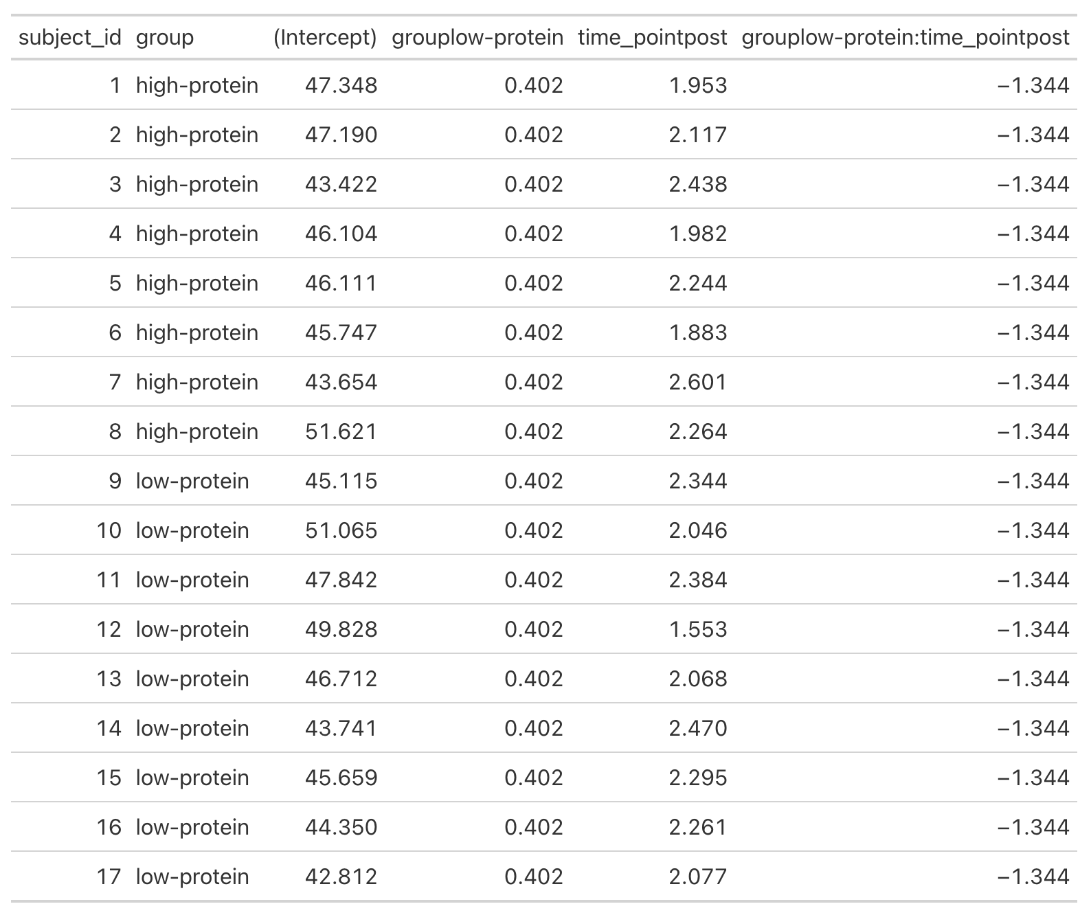
- We can plot each subjects random effects intercept posterior distribution (see GITHUB code)
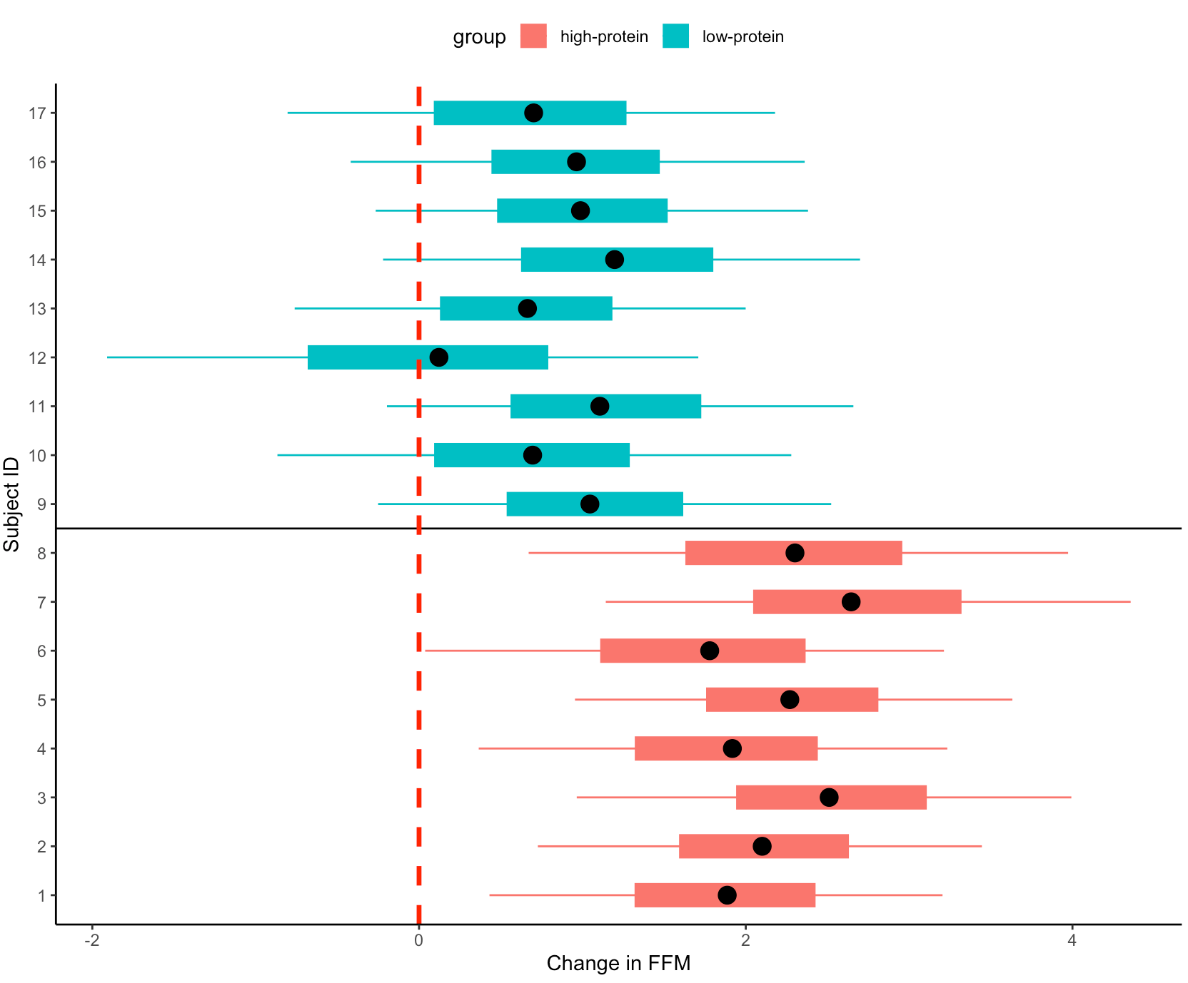
- We can plot each subjects random slope posterior distribution (see GITHUB code)
- Finally, we can get predicted values from the model for the pre- and post-test FFM for each subject, based on their group.
- We will use `posterior_epred()` to do this, which provides us with uncertainty around the average value, helping us to visualize the uncertainty around our model estimates. This is different than if we were to use `posterior_preidct()`, which also incorporates observation-level noise and is good simulating raw data on a *hypothetical* new person who we are trying to make an inference on.
Repeating the simulation
- Okay, that is all interesting. We can see how the simulation returned the results of the ground truth coefficients that we set up. We can also see how the Bayesian mixed model was useful in helping us say more than just *”This group was better than that group”* by allowing us to extract posterior draws, visualize our uncertainty and, if we wanted, make more substantive statements about the individual subjects in our study.
- The next thing we need to consider is the notion that this was one study with 17 subjects. If we pulled 17 new subjects, perhaps the results would look different? So, let’s set up a `for()` loop to play out 1000 simulated studies of the same data. We will keep the ground truth coefficients for the fixed effects the same as above — but of course you can allow them to vary if you’d like. In the loop, with each study, we will allow our subject intercepts and our model error to vary since we wouldn’t expect those to be the same if we selected a new group of 17 subjects. For each simulation we will simply extract the group*time interaction coefficient, since that is what we care about from the study.
NOTE: For purposes of time, we will use {lme4} to calculate the mixed models so that we don’t have to run 1000 Markov Chain Monte Carlo Simulations (as we would if we did a Bayesian mixed model like above).
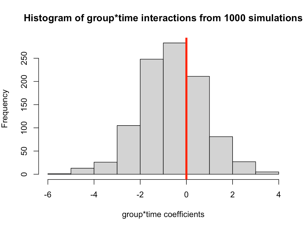

- In simulating this 1000 times we see that the median value is around where we specified it, 0.6 (the ground truth). However, we see considerable variability in this effect over the 1000 simulations. This could be because of the amount of variability that I have in the subject intercepts and the model error. Someone who does this type of research all of the time might have a better/more plausible prior assumption of what type of variability we would expect for these parameters. The point, however, is that one study is simply a snapshot of a small population that we hope to learn from and infer something meaningful to the broader population. Had the study been done again with a different group of 17 female physique competitors we might have gotten totally different results.
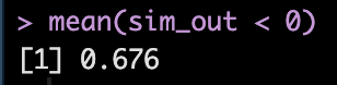
- Overall, the effect does still favor the high-protein group with 68% of the distribution below 0, indicating a positive effect on fat free mass for high-protein relative to low protein.