A friend of mine was downloading some force plate data from the software provider so that he could evaluate test data in a few of his athletes during return to play. The issue he was running into was that the different athletes all had different numbers of tests and different start and end testing times. The software exports the test outputs by date and he was wondering how he could normalize the dates to numeric values (e.g. Test 1, Test 2, etc.) so that he could model the date (since we can’t really use a Date in a regression model).
I’ll be the first to admit that working with dates and times can be an incredible pain in the butt. For reference, I covered the topic of converting Catapult GPS practice duration strings to actual training minutes, HERE. To help him out, I provided a few different solutions depending on the research question. I also add some code for calculating changes in test performance between tests and from each test to baseline.
The full code is available on my GITHUB page.
Loading Packages & Simulating Data
## load packages ----------------------------------------------
library(tidyverse)
library(lubridate)
## Simulate data ----------------------------------------------
set.seed(78)
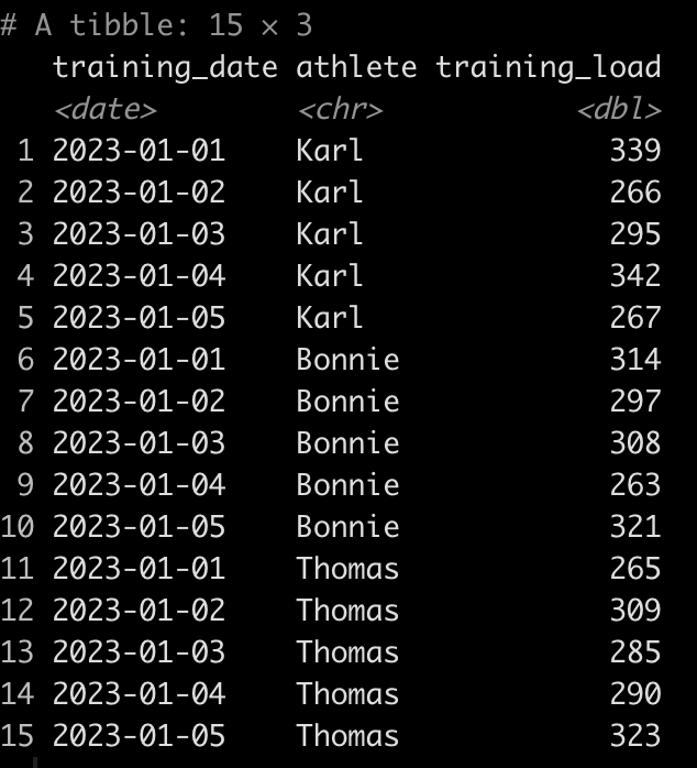
dat <- tibble(
athlete = rep(c("Tom", "Bob", "Franklin"), times = c(5, 10, 3)),
test_dates = c(
seq(as.Date("2023-01-01"), as.Date("2023-01-5"), by = "days"),
seq(as.Date("2023-02-15"), as.Date("2023-02-24"), by = "days"),
as.Date(c("2023-01-19", "2023-01-30", "2023-02-26"))
),
jump_height = round(rnorm(n = 18, mean = 28, sd = 2.5), 1)
)
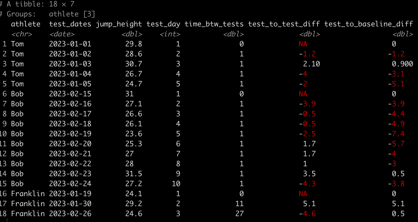
dat
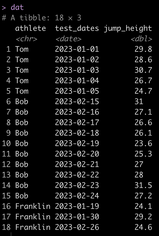
We can see that Tom has 5 tests, Bob has 10, and Franklin has only 3. Additionally, Tom and Bob tested every day, consecutively, while Franklin was less compliant and has larger time frames between his tests.
Create a test number
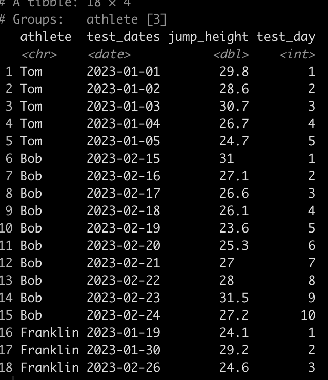
First, let’s normalize the Dates so that they are numeric. Basically, instead of dates we want a value indicating whether the test was test 1, or test 5, or test N. We will do this by creating a row_number() id/counter for each individual athlete.
### Create a test number ------------------------------------------
dat <- dat %>%
  group_by(athlete) %>%
  mutate(test_day = row_number())

dat
Calculating the time between tests
Alternatively, we may not just want to know the test number of each test but we may want to determine the amount of days between each test.
The code to do this is a bit ugly looking so let’s unpack it.
- Since we are dealing with dates we use the difftime() function which takes an argument for the two times you are looking to calculate the difference between. Here, we are trying to calculate the difference in time (days) between one date and the date preceding it for each individual athlete.
- The difftime() function will produce a to time variable. If we want to make this numeric we need to convert it to a character so we do that with the as.character() function.
- Once the variable is a character we use the as.numeric() function to convert it to a numeric value.
- Finally, since the first value for each athlete will be an NA, since there is no date preceding the first test, we use the coalesce() function to fill in a 0 value for each of the NA’s, to indicate that this was the first test and thus there was no time between it and any other test.
### Calculate the time between tests -------------------------------
dat <- dat %>%
  group_by(athlete) %>%
  mutate(time_btw_tests = coalesce(as.numeric(as.character(difftime(test_dates, lag(test_dates)))), 0))

dat
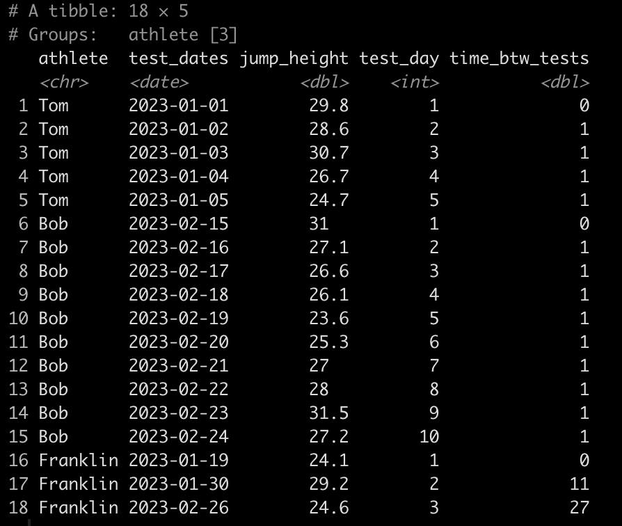
Notice that Tom and Bob have 1 day between all of their tests while Franklin’s second test was 11 days after his first and his third test was 27 days after his second.
Calculate the difference in jump height from one test to the next
### Calculate difference in jump height from one day to the next -------------------
dat <- dat %>%
  group_by(athlete) %>%
  mutate(test_to_test_diff = jump_height - lag(jump_height))

dat

Here, we use the lag() function to calculate the difference in one value from the value before it within in the same column. Since we grouped by athlete, which is what we want, their first test will always have an NA, in this new column, since there was no test preceding it.
Calculating the difference in jump height from the baseline test
Finally, we might also be interested to evaluate the performance on each test relative to the athlete’s baseline test. To do this we simply subtract jump_height from the jump_height indexed in row one for each athlete.
### Calculate difference in jump height from each test to the baseline test -------------

dat <- dat %>%
  group_by(athlete) %>%
  mutate(test_to_baseline_diff = jump_height - jump_height[1])

dat
Wrapping Up
Dates and times are always tricky to deal with. Most of the sports technology providers will proved data as dates (or unix timestamps) meaning that we have to do some cleaning of the data to codify the dates as numeric values representing the test number or the days between tests (depending on the research question). Additionally, using lag functions can be helpful for calculating he difference from one test to the next or from each test to the baseline.
The entire code is available on my GITHUB page.
If you have any data cleaning issues that you are dealing with from various sports science technologies, feel free to reach out!