
A colleague recently asked me a good question regarding some feature engineering for some data he was working with. He was collecting training load data and wanted to create a z-score for each observation, BUT, he didn’t want the most recent observation to be included into the calculation of the mean and standard deviation. Basically, he wanted to represent the z-score for the most recent observation normalized to the observations that came before it.
This is an interesting issue because it makes me think of sports science research that uses z-scores to calculate the relationship between training load and injury. If the z-score is calculated retrospectively on the season then the observed z-scores and their relationship to the outcome of interest (injury) is a bit misleading as the mean and standard deviation of the full season data is not information one would have had on the day in which the injury occurred. All the practitioner would know, as the season progresses along, is the mean and standard deviation of the data up to the most recent observation.
So, let’s calculate some lagged mean and standard deviation values! The full code is available on my GITHUB page.
Loading Packages and Simulating Data
Aside from loading {tidyverse} we will also load the {zoo} package, which is a common package used for constructing rolling window functions (this is useful as it prevents us from having to write our own custom function).
We will start with a simple data set of just 10 training load observations.
## Load Libraries
library(tidyverse)
library(zoo)

## Simulate Data
set.seed(45)
d <- tibble(
  day = 1:10,
  training_load = round(rnorm(n = 10, min = 250, max = 350), 0)
)

d

Calculate the z-score with the mean and standard deviation of all data that came before it
To do this we use the rollapplyr() function from the {zoo} package. If we want to include the most recent observation in the mean and standard deviation we can run the function as is. However, because we want the mean and standard deviation of all data previous to, but not including, the most recent observation we wrap this entire function in the lag() function, which will take the data in the row directly above the recent observation. The width argument indicates the width of the window we want to calculate the function over. In this case, since we have a day variable we can use that number as our window width to ensure we are getting all observed data prior to the most recent observation.
d <- d %>%
  mutate(lag_mean = lag(rollapplyr(data = training_load, width = day, FUN = mean, fill = NA)),
         lag_sd = lag(rollapplyr(data = training_load, width = day, FUN = sd, fill = NA)),
         z_score = (training_load - lag_mean) / lag_sd)

d
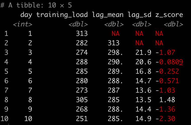
This looks correct. As a sanity check, let’s calculate the mean and standard deviation of the first 4 rows of training load observations and see if those values correspond to what is in the lag_mean and lag_sd columns at row 5.
first_four <- d %>%
  slice(1:4) %>%
  pull(training_load)

mean(first_four)
sd(first_four)
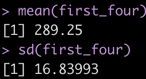
It worked!
A more complicated example
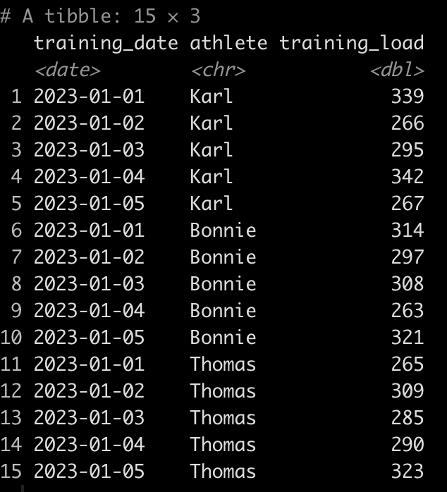
Okay, that was an easy one. We had one athlete and we had a training day column, which we could use for the window with, already built for us. What if we have a data set with multiple athletes and only training dates, representing the day that training happened?
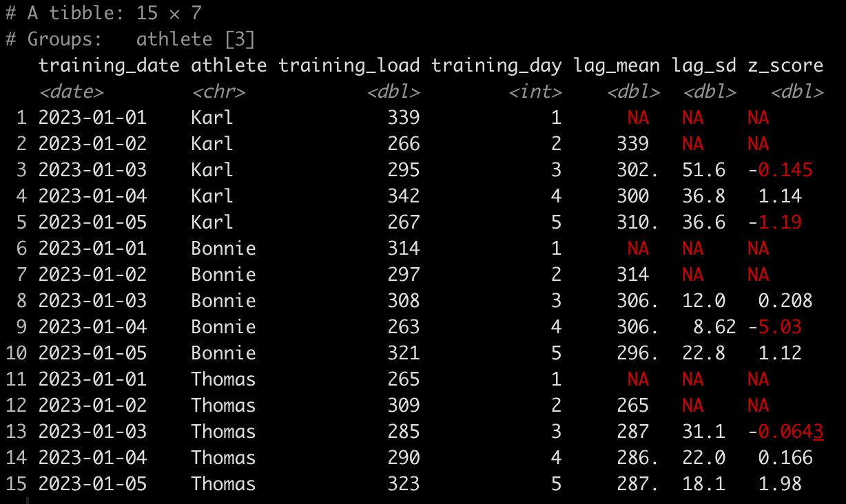
To make this work we will group_by() the athlete, and use the row_number() function to calculate a training day variable that represents our window width. Then, we simply use the same code above.
Let’s simulate some data.
set.seed(67)
d <- tibble(
  training_date = rep(seq(as.Date("2023-01-01"),as.Date("2023-01-05"), by = 1), times = 3),
  athlete = rep(c("Karl", "Bonnie", "Thomas"), each = 5),
  training_load = round(runif(n = 15, min = 250, max = 350), 0)
)

d
Now we run all of our functions for each athlete.
d <- d %>%
  group_by(athlete) %>%
  mutate(training_day = row_number(),
         lag_mean = lag(rollapplyr(data = training_load, width = training_day, FUN = mean, fill = NA)),
         lag_sd = lag(rollapplyr(data = training_load, width = training_day, FUN = sd, fill = NA)),
         z_score = (training_load - lag_mean) / lag_sd)


d
Wrapping Up
There we have it, a simple way of calculating rolling z-scores while using the mean and standard deviation of the observations that came before the most recent observation!
If you’d like the entire code, check out my GITHUB page.