One of the most frustrating things to deal with is date and time strings. Using Catapult GPS, a popular GPS provider for professional and collegiate sports teams, practice duration is reported in their export as a string, hours : minutes : seconds. Unfortunately, we can’t do much with this if we want to perform additional computations, for example calculate player load per minute, we need to convert this column into total minutes.
I’ve had a few people in the sports performance field reach out and ask how to do this in R because they often get frustrated and just resort to changing the data in their CSV download prior to importing it into R, where they then do their plotting and visualizing. Today, I’ll walk through a few steps using the {lubridate} package and show you how you can handle this data cleaning all within you R environment.
Load Packages & Get Data
We start by loading {tidyverse} and {lubridate} and some fake Catpault data that I’ve created.
### Packages ---------------------------------------
library(tidyverse)
library(lubridate)

### Load Data -------------------------------------
catapult <- read.csv("catapult_example.csv", header = TRUE) %>%
janitor::clean_names()

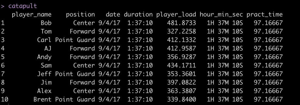
catapult
Adjusting time
We can see the duration string (hour : minute : second) indicating that the session was 97 minutes and 10 seconds long. Before handling the entire column of data, let’s just grab a single observation and work through the functions we need so that we know what is going on.
### Adjust Time ------------------------------------
# hms() function to split out duration to its component parts into a string
single_time <- catapult %>%
  slice(1) %>%
  pull(duration)

single_time
The hms() function can be used to convert each of the time components into a named string.
single_time2 <- hms(single_time)
single_time2
 Once we have the individual components in a named string we can extract them out with the hour(), minute(), and second() functions and have each returned back as an integer.
# Select each component
hour(single_time2)
minute(single_time2)
second(single_time2)
Once in integer form, converting this data to a total minutes value we first multiplying hour by 60 and divide second by 60 and then sum those up with minutes.
hour(single_time2)*60 + minute(single_time2) + second(single_time2)/60

The finished product suggests the session was 97.2 minutes long.
Applying the approach to all of our data
Now that we understand what is going on under the hood, we can apply this at scale, to our of our data.
catapult <- catapult %>%
  mutate(hour_min_sec = hms(duration),
    pract_time = hour(hour_min_sec) * 60 + minute(hour_min_sec) + second(hour_min_sec) / 60)

catapult
After getting practice time into minutes we will adjust the date column from a character string to an actual date, using the as.Date() function.
catapult$date <- as.Date(catapult$date, "%m/%d/%y")
catapult
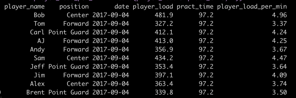
To finish, we will do a bit of clean up and remove the duration and hour_min_sec columns, round the player_load and pract_time columns to one significant digit and create a player_load_per_min column.
catapult %>%
  select(-duration, -hour_min_sec) %>%
  mutate(across(.cols = player_load:pract_time,
                ~round(.x, 1)),
         player_load_per_min = round(player_load / pract_time, 2))
Now we have a cleaned data set that we can worth with!
Access to the full code is available on my GITHUB page.


