Workflowsets in {tidymodels} provide a useful way for analysts to run several models, even tune several machine learning models on their dataset, simultaneously. You can then extract model fit information, predictions, and make comparisons to identify the most effective model type and the optimized tuning parameters.

Below are links to two workflowsets tutorials I’ve written. The first link is to an older tutorial that wrote and posted in the blog 3 months ago. This tutorial builds several machine learning models on NWSL data to solve a classification task. The second link is a more recent tutorial that walks through workflowsets and model tuning for outcomes that are both binary and continuous.

Both tutorials go over model building, hyperparameter tuning, model comparisons, making predictions, and storing the final model for deployment at a later time in {tidymodels} using workflowsets.

Hopefully both tutorials provide analysts with a clear overview of how to set up workflowsets and run several models in parallel, helping to make their work more efficient.

Tutorial 1

Tutorial 2

We’ve been working on building simulations in R over the past few articles. We are now to the point where we want to simulate data using regression models. To recap what we’ve done so far:

• Part 1 discussed the basic functions for simulating and sampling data in R.
• Part 2 walked us through how to perform bootstrap resampling and then simulate bivariate and multivariate distributions.
• Part 3 we worked making group comparisons by simulating thousands of t-tests

In an upcoming article we will use simulation to evaluate regression assumptions. But, before we do that, it might be useful to use a regression model reported in a research paper to simulate a data set. This can be useful if you are trying to better understand the paper (you can recalculate statistics and explore the data) or if you want to work on applying a different type of model approach to build hypotheses for future research.

As always, all code is freely available in the Github repository.

I’m going to take the regression model from a paper by Ferrari et al (2022), Performance and anthropometrics of classic powerlifters: Which characteristics matter? J Strength Cond Res., which looked to predict power lifting performance in male and female lifters.

The paper used several variables to try and predict Squat, Bench, Deadlift, and Powerlifting Total in raw power lifters. To keep this simple, I’ll focus on the model for predicting squat performance, which was:

The model had a standard error of estimate (SEE) of 20.3 and an r-squared of 0.83.

Getting the necessary info from the paper

Aside from the model coefficients, above, we also need to get the mean and standard deviation for each of the variables in the model (for both male and female lifters). We will use those parameters to simulate 1000 male and female lifters.

library(tidyverse)

# set the see for reproducibility
set.seed(82)

# sample size - simulate 1000 male and 1000 female lifters
n_males <- 1000
n_females <- 1000

# set the model coefficients for squats
intercept <- -145.7
years_exp_beta <- 4.3
pct_bf_beta <- -1.7
upper_arm_girth_beta <- 6
thigh_girth_beta <- 1.9

# Standard Error of Estimate (SEE) is sampled from a normal distribution with a mean = 0 and 
# standard deviation of 20.3
see <- rnorm(n = n_males + n_females, mean = 0, sd = 20.3)

# get mean and sd for each of the model variables
years_exp_male <- rnorm(n = n_males, mean = 2.6, sd = 2.4)
years_exp_male <- ifelse(years_exp_male < 0, 0, years_exp_male)
years_exp_female <- rnorm(n = n_females, mean = 1.6, sd = 1.5)
years_exp_female <- ifelse(years_exp_female < 0, 0, years_exp_female)
pct_bf_male <- rnorm(n = n_males, mean = 11.1, sd = 3.8)
pct_bf_female <- rnorm(n = n_females, mean = 21.7, sd = 5.4)
upper_arm_girth_male <- rnorm(n = n_males, mean = 35.6, sd = 2.8)
upper_arm_girth_female <- rnorm(n = n_females, mean = 29.5, sd = 3.1)
thigh_girth_male <- rnorm(n = n_males, mean = 61.1, sd = 5.5)
thigh_girth_female <- rnorm(n = n_females, mean = 56.1, sd = 4.9)

# put the simulated data into a data frame
dat <- data.frame( gender = c(rep("male", times = n_males), rep("female", times = n_females)), years_exp = c(years_exp_male, years_exp_female), pct_bf = c(pct_bf_male, pct_bf_female), upper_arm_girth = c(upper_arm_girth_male, upper_arm_girth_female), thigh_girth = c(thigh_girth_male, thigh_girth_female) ) dat %>%
  head()

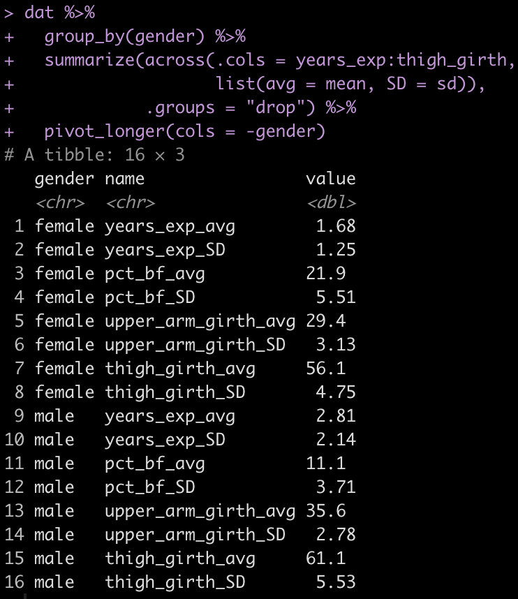
As a sanity check, we can quickly check the mean and standard deviation of each variable to ensure the simulation appears as we intended it to.

## check means and standard deviations of the simulation
dat %>%
  group_by(gender) %>%
  summarize(across(.cols = years_exp:thigh_girth,
                   list(avg = mean, SD = sd)),
            .groups = "drop") %>%
  pivot_longer(cols = -gender)

Estimate squat performance using the model

Next, we use the values that we simulated and the model coefficients to simulate the outcome of interest (Squat performance).

# estimate squat performance
dat$squat <- with(dat, intercept + years_exp_beta*years_exp + pct_bf_beta*pct_bf + upper_arm_girth_beta*upper_arm_girth + thigh_girth_beta*thigh_girth + see) dat %>%
  head()

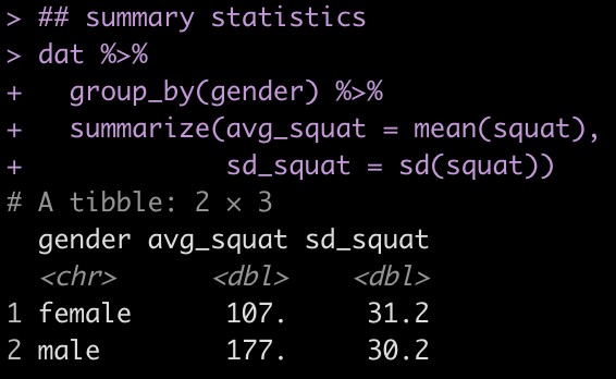
## summary statistics
dat %>%
  group_by(gender) %>%
  summarize(avg_squat = mean(squat), 
            sd_squat = sd(squat))

# plots
hist(dat$squat)

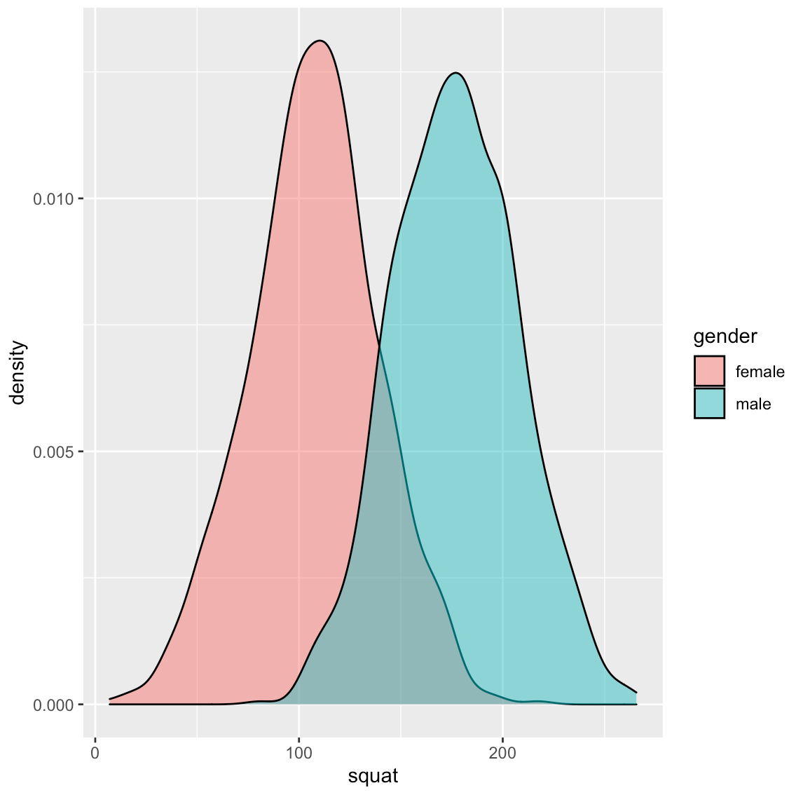
dat %>%
  ggplot(aes(x = squat, fill = gender)) +
  geom_density(alpha = 0.5)

Look at the regression model

Now we fit a regression model with our simulated data.

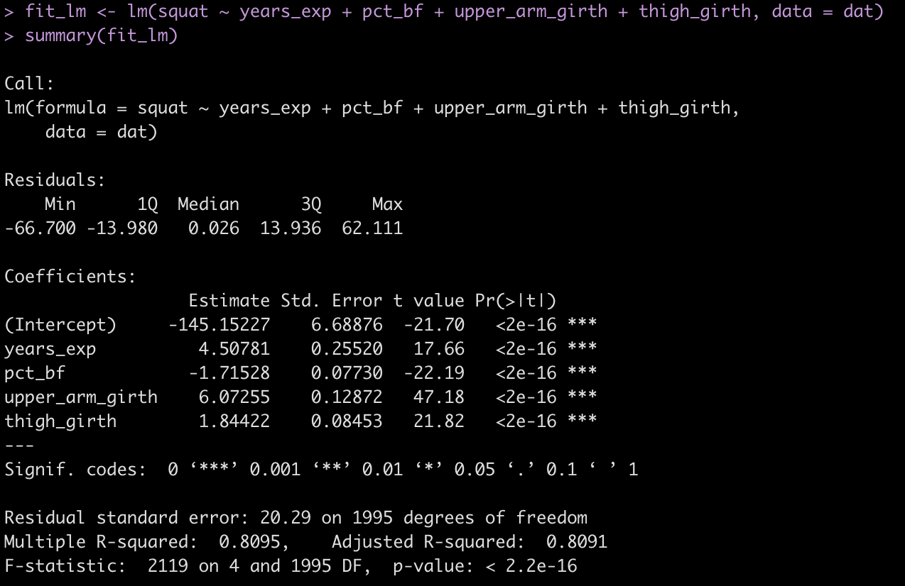
fit_lm <- lm(squat ~ years_exp + pct_bf + upper_arm_girth + thigh_girth, data = dat)
summary(fit_lm)

• The coefficients are similar to those in the paper (which makes sense because we coded them this way.
• The standard error (Residual standard error) is 20.3, as expected.
• The r-squared for the model is 0.81, close to what was observed in the paper.

Making a better simulation

One thing to notice is the mean and standard deviation of the squat in our simulation is a bit less compared to what is reported for the population in the paper.

Our estimates are a little low relative to what was reported in the paper. The model above still works because we constructed it with the regression coefficients and variable parameters in the model, so we can still play with the data and learn something. But, the estimated squats might be a little low because the anthropometric variables in the model (BF%, Upper Arm Girth, and Thigh Girth) are in some way going to be correlated with each other. So, we could make this simulation more informative by simulating those variables from a multivariate normal distribution, as we did in Part 3.

To start, we load the mvtnorm package and set up a vector of mean values for each variable. We will construct a vector for males and females separately. We will use the mean values for each variable reported in the paper.

library(mvtnorm)

## Order of means is: BF%, Upper Arm Girth, Thigh Girth
male_means <- c(11.1, 35.6, 61.1)
female_means <- c(21.7, 29.5, 56.1)

Next, we need to construct a correlation matrix between these three variables. Again, we will create a correlation matrix for males and females, separately. I’m not sure of the exact correlation between these variables, so I’ll just estimate what I believe it to be. For example, the correlations probably aren’t 0.99 but they also probably aren’t below 0.6. I’m also unsure how these correlations might differ between the two genders. Thus, I’ll keep the same correlation matrix for both. To keep it simple, I’ll set the correlation between BF% and upper arm and thigh girth at 0.85 and the correlation between upper arm girth and thigh girth to be 0.9. In theory, we could consult some scientific literature on these things and attempt to construct more plausible correlations.

## Create correlation matrices
# males
male_r_matrix <- matrix(c(1, 0.85, 0.85,
                          0.85, 1, 0.9,
                          0.85, 0.9, 1), 
                   nrow = 3, ncol = 3,
       dimnames = list(c("bf_pct", "upper_arm_girth", "thigh_girth"),
                       c("bf_pct", "upper_arm_girth", "thigh_girth")))

male_r_matrix

# females
female_r_matrix <- matrix(c(1, 0.85, 0.85,
                          0.85, 1, 0.9,
                          0.85, 0.9, 1), 
                   nrow = 3, ncol = 3,
       dimnames = list(c("bf_pct", "upper_arm_girth", "thigh_girth"),
                       c("bf_pct", "upper_arm_girth", "thigh_girth")))

female_r_matrix

Now we will create 1000 simulations from a multivariate normal distribution for both males and females and then row bind them together into a single big data frame.

## simulate 1000 new x, y, and z variables using the mvtnorm package
set.seed(777)
male_sim <- rmvnorm(n = n_males, mean = male_means, sigma = male_r_matrix) %>%
  as.data.frame() %>%
  setNames(c("pct_bf", "upper_arm_girth", "thigh_girth"))

female_sim <- rmvnorm(n = n_females, mean = female_means, sigma = female_r_matrix) %>%
  as.data.frame() %>%
  setNames(c("pct_bf", "upper_arm_girth", "thigh_girth"))

head(male_sim)
head(female_sim)

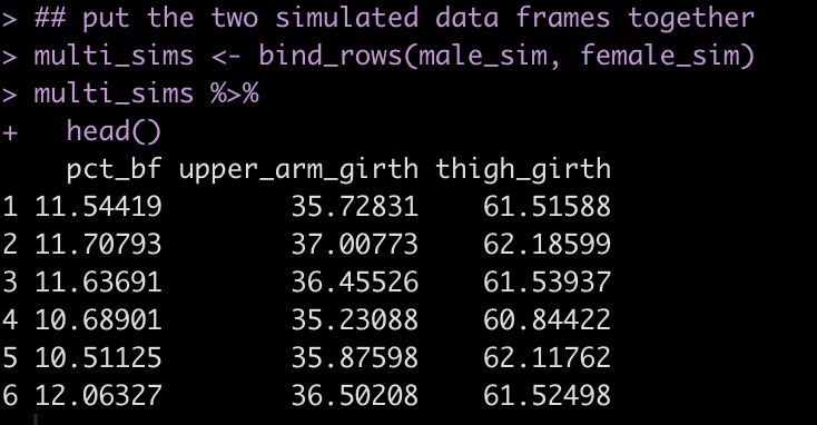
## put the two simulated data frames together
multi_sims <- bind_rows(male_sim, female_sim) multi_sims %>%
  head()

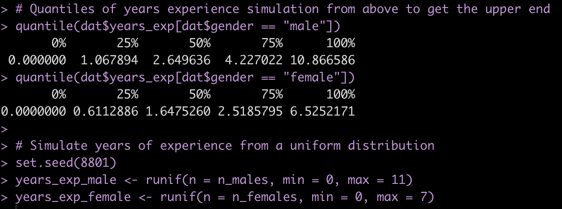
Finally, one last thing we’ll change is our simulation of years of experience. This variable is not a normally distributed variable because it is truncated at 0. Above, in our first simulation, we attempted to solve this with the ifelse() expression to assign any simulated value less than 0 to 0. Here, I’ll just get the quantiles of the simulated years of experience so that I have an idea of a plausible upper end of experience for the population used in this paper. Then, instead of simulating from a normal distribution I’ll do a random draw from a uniform distribution from 0 to the respective upper end for the male and female groups.

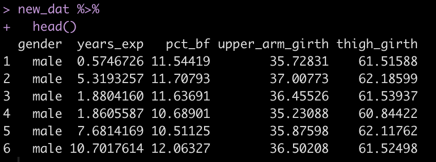
Now take the newly simulated variables and create a new data frame.

## new data frame
new_dat <- data.frame( gender = c(rep("male", times = n_males), rep("female", times = n_females)), years_exp = c(years_exp_male, years_exp_female) ) %>%
  bind_cols(multi_sims)

new_dat %>%
  head()

Finally, go through the steps we did above to estimate the squat from our four variables and the beta coefficients from the paper.

# estimate squat performance
new_dat$squat <- with(new_dat, intercept + years_exp_beta*years_exp + pct_bf_beta*pct_bf + upper_arm_girth_beta*upper_arm_girth + thigh_girth_beta*thigh_girth + see) new_dat %>%
  head()

## summary statistics
new_dat %>%
  group_by(gender) %>%
  summarize(avg_squat = mean(squat), 
            sd_squat = sd(squat))

# plots
hist(new_dat$squat)

new_dat %>%
  ggplot(aes(x = squat, fill = gender)) +
  geom_density(alpha = 0.5)

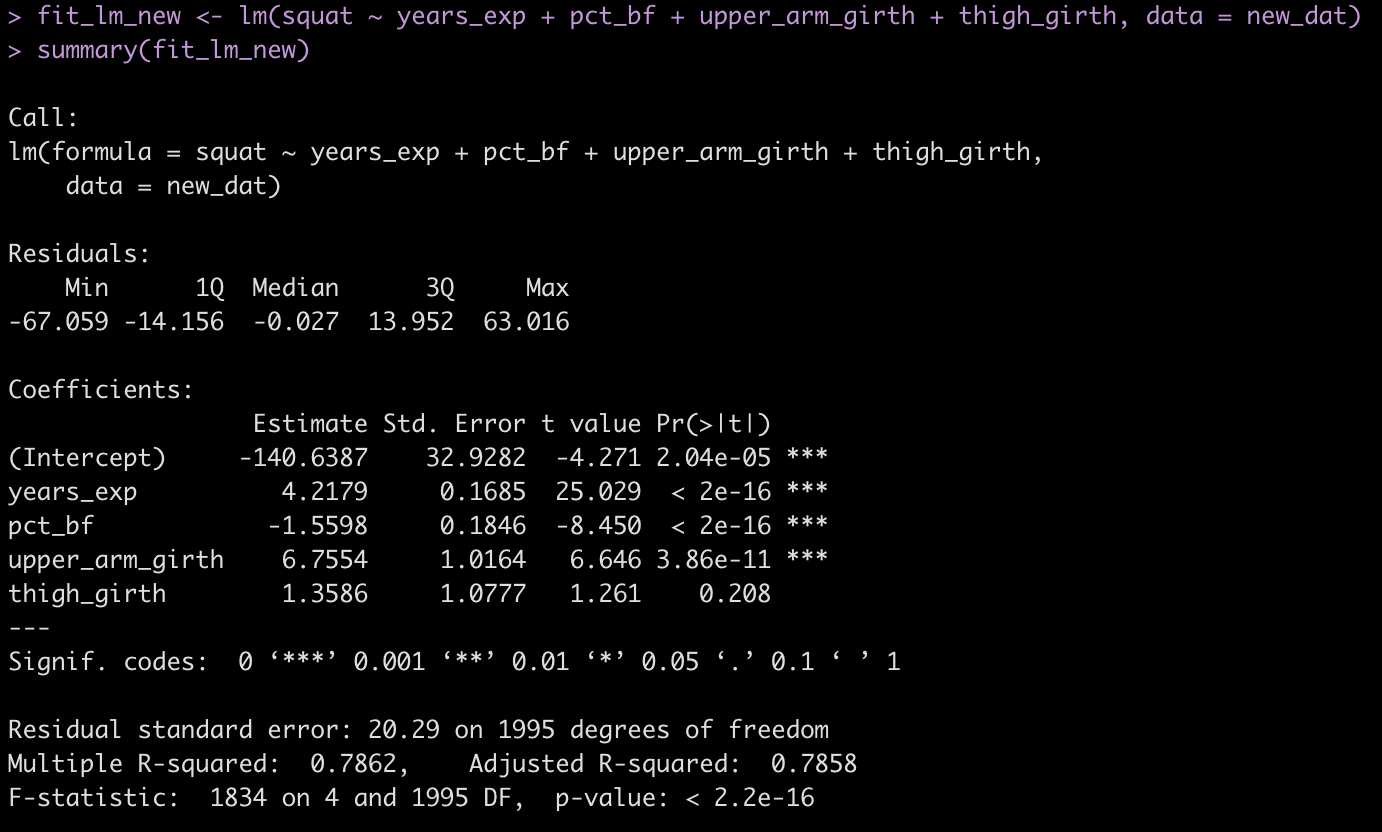
Look at the new regression model

fit_lm_new <- lm(squat ~ years_exp + pct_bf + upper_arm_girth + thigh_girth, data = new_dat)
summary(fit_lm_new)

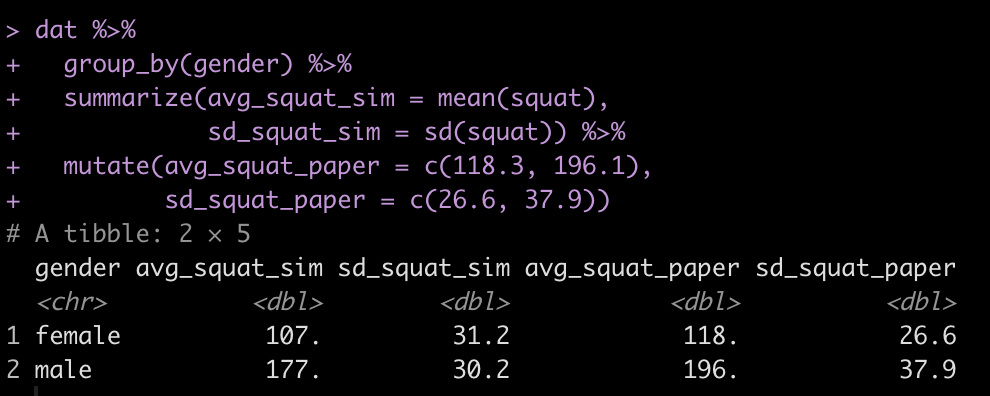
Compare the squat simulated data to that which was reported in the paper

new_dat %>%
  group_by(gender) %>%
  summarize(avg_squat_sim = mean(squat), 
            sd_squat_sim = sd(squat)) %>%
  mutate(avg_squat_paper = c(118.3, 196.1),
         sd_squat_paper = c(26.6, 37.9))

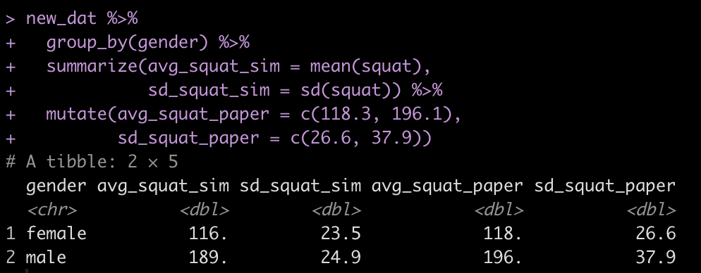
Now we have mean values much closer to those observed in the population of the study. Our standard deviations differ from the study because, if you recall, the standard error of the estimate was 20.3 for the regression model. The model in the study did not include gender as an independent variable. This to me is a little strange and in the discussion of the paper the authors’ also indicate that it was strange to them too. However, the approach the authors’ took to building this deemed gender unnecessary as a predictor variable. Consequently, our simulation has a similar standard deviation in estimate squat for both the male and female populations. However, we now have a data set that is relatively close to what was observed in the paper and can therefore proceed with conducting other statistical tests or building other models.

Wrapping Up

We’ve come a long way in our simulation journey, from randomly drawing single vectors of data to now building up entire data sets using regression models and simulating data from research studies. Next time we will use simulation to explore regression assumptions.

As always, all code is freely available in the Github repository.

To review where we are at so far:

• Part 1 discussed the basic functions for simulating and sampling data in R.
• Part 2 walked us through how to perform bootstrap resampling and then simulate bivariate and multivariate distributions.

In Part 3, we are ready to put this info to use and start to simulate data and construct models. To start things off, this tutorial will focus on simulating data for comparison of group means — a t-test.

As always, all code is freely available in the Github repository.

Simulating Two Groups for Comparison

We begin by simulating two groups using the rnorm() function to make a random draw from a normal distribution. Group 1 will have a mean of 50 and a standard deviation of 10 while Group 2 will have a mean of 60 with a standard deviation of 6.25. Both groups have a sample size of 10 (so this is a small study!).

In addition to simulating the data, we will store summary statistics for each group so that we can use them later.

set.seed(1759)
grp1 <- rnorm(n = 10,
              mean = 50,
              sd = 10)

grp2 <- rnorm(n = 10,
              mean = 60,
              sd = 6.25)

## get the summary statistics for both groups
# sample size
n_grp1 <- length(grp1)
n_grp2 <- length(grp2)

# means
mu_grp1 <- mean(grp1)
mu_grp2 <- mean(grp2)

# variances
var_grp1 <- var(grp1)
var_grp2 <- var(grp2)

# standard deviation
sd_grp1 <- sd(grp1)
sd_grp2 <- sd(grp2)

Next, we calculate the t-statistic, which is the difference between the two groups means divided by the pooled standard deviation of the two groups.

## pooled SD
sd_pool <- sqrt(((n_grp1 - 1) * var_grp1 + (n_grp2 - 1) * var_grp2) / (n_grp1 + n_grp2 - 2))
sd_pool

## Compute t-statistic
t_stat <- (mu_grp1 - mu_grp2) / (sd_pool * sqrt(1/n_grp1 + 1/n_grp2))
t_stat

We can use this t-statistic to determine if the difference is significant or not at a desired alpha level, say p < 0.05, by using a t-distribution (the qt() function, which we were introduced to in Part 1 of this series). We then check our work against R’s build in t.test() function.

alpha <- 0.05
df <- n_grp1 + n_grp2 - 2 if(abs(t_stat) > qt(1 - alpha / 2, df, lower.tail = TRUE)){
  "significant difference"} else {"not a significant difference"} 

# Get p-value
p_value <- 2*pt(abs(t_stat), df, lower=FALSE)
p_value

# check work
t.test(grp1, grp2)

The group difference is barely significant at the p < 0.05 level. We calculated the t-statistic by hand and got the exact same value as that which was produced by the t.test() function.

To make this approach more streamlined, let’s create our own t-test function so that all we need to do in the future is pass it a vector of values representing each group’s data and get returned the t-statistic.

## t-test function
t_stat_func <- function(x, y){
  n_grp1 <- length(x)
  n_grp2 <- length(y)
  sd_pool <- sqrt(((n_grp1 - 1) * sd(x)^2 + (n_grp2 - 1) * sd(y)^2) / (n_grp1 + n_grp2 - 2))
  t_stat <- (mean(x) - mean(y)) / (sd_pool * sqrt(1/n_grp1 + 1/n_grp2))
  return(t_stat)
}

## try out the function
t_stat_func(x = grp1, y = grp2)

We only have 10 observations in each of our groups. With such a small sample size, it may be challenging to really know if the difference we observed is real or just some sort of chance/luck occurrence (we will explore sample size issues via simulation in a later blog post). What we can do is use the function we just created and build simulated distributions using the data generating process (mean and SD) of each group to run a Monte Carlo simulations and explore how often we might reject or accept the null hypothesis at an alpha level of p < 0.05.

# Let's set alpha to 0.05
alpha <- 0.05

# We will run 10,000 simulations
N_sims <- 1e4

# create an empty vector for storing t-statistics and p-valies
t_stat <- rep(NA, N_sims)
p_values <- rep(NA, N_sims)

for(i in 1:N_sims){
  
  # simulate population 1
  grp1_sim <- rnorm(n = n_grp1, mean = mu_grp1, sd = sd_grp1)
  
  # simulate group 2
  grp2_sim <- rnorm(n = n_grp2, mean = mu_grp2, sd = sd_grp2)
  
  # compute the t-statistic with our function
  t_stat[i] <- t_stat_func(grp1_sim, grp2_sim)

  # get degrees of freedom for calculating the p-value
  df <- n_grp1 + n_grp2 - 2
  
  # obtain the p-value
  p_value[i] <- 2*pt(abs(t_stat[i]), df, lower=FALSE)
}

par(mfrow = c(1, 2))
hist(abs(t_stat),
     main = "T-Statistic Distribution")
abline(v = mean(abs(t_stat)),
       col = "red",
       lwd = 3,
       lty = 2)
hist(p_value,
     main = "p-value Distribution")
abline(v = 0.05,
       col = "red",
       lwd = 3,
       lty = 2)

# What percentage of times did we reject the null?
mean(p_value < 0.05)

You will get slightly different results, since I didn’t set a seed, but you will find that we end up rejecting the null about 52-53% of the time, meaning we probably wouldn’t want to be too confident about our “statistically significant” finding.

We could have saved a lot of lines of code and instead used the replicate() function and run 10,000 simulations of the t-test between the two groups (additionally, replicate() will run faster than the for() loop).

t_test <- function(){
  grp1 <- rnorm(n = n_grp1, mean = mu_grp1, sd = sd_grp1)
  grp2 <- rnorm(n = n_grp2, mean = mu_grp2, sd = sd_grp2)
  t_stat_func(grp1, grp2)
}


# Instead of a for loop, we will use the replicate() function to run this 10,000 times
t_stat_vector <- replicate(n = 10000,
                           t_test())

head(t_stat_vector)
hist(abs(t_stat_vector),
     main = "T-Test Simulation using replicate()",
     xlab = "T-Statistic")

Simulating Data from Studies

Why just create fake data and play around when we can use a similar approach to simulating data to help us further explore data contained in studies we read?! Most studies do not provide full data sets but do provide necessary summary statistics (e.g., sample size, mean, standard deviation, standard errors, confidence intervals, etc.), allowing us to use the data generating processes to simulate the study.

I was reading a 2010 paper from Saenz et al., Knee isokinetic test-retest: A multicenter knee isokinetic test-retest study of a fatigue protocol (Eur J Phys Rehabil Med), where they authors were conducing a series of test-retest protocols using a biodex. The tables in the paper lay out the information required to simulate the study. For example, in Table 1, the authors’ provide the mean, median, and standard deviation for all of the extension tests that were performed. I’ll use the data provided for the test, WRepMax.

## Saenz (2010) - Knee isokinetic test-retest - simulation
## Table 1: Extension
# We will simulate the test scores provided for WrepMax

# number of subjects
N <- 90

## Get the mean and SD for the test and retest from Table 1 for WrepMax
test1_mu <- 99.3
test1_sd <- 18.34
test2_mu <- 104.44
test2_sd <- 24.90

Next, we calculate the mean difference between test 1 and test 2 and grab the standard deviation for the test, provided in Table 3 of the paper.

## Get the difference and standard deviation of the difference between test 1 and 2 from Table 3 (row 1)
diff <- test1_mu - test2_mu
sd_diff <- 17.37

First, we simulate Test 1 using the above parameters (sample size, mean, and standard deviation).

## Simulate the first test using the summary statistics from Table 1
set.seed(925)
w_rep_max_1 <- rnorm(n = N, mean = test1_mu, sd = test1_sd)

Next, we simulate Test 2. However, we have to remember consider that, because we are trying to simulate the performance of the 90 participant in the study, Test 2 has a relationship to the performance of Test 1 because the authors’ are analyzing the difference in performance between the two tests. Therefore, to create Test 2 we will use our simulation of Test 1 for each participant and include some random error, which is specific to the mean and standard deviation of the difference between Test 1 and Test 2 reported in the study.

## Simulate test 2 by taking test 1 and applying the observed difference between tests (Table 3) 
set.seed(479)
w_rep_max_2 <- w_rep_max_1 + rnorm(n = N, mean = abs(diff), sd = sd_diff)

Now that we have Test 1 and Test 2 simulated for each participant, we can calculate the summary statistics and see how well they compare to the observed data reported in the study.

## Get the mean and SD of the simulated test1 and test 2
test1_mu_sim <- mean(w_rep_max_1) 
test1_sd_sim <- sd(w_rep_max_1)

test2_mu_sim <- mean(w_rep_max_2)
test2_sd_sim <- sd(w_rep_max_2)

test1_mu_sim
test1_sd_sim

test2_mu_sim
test2_sd_sim

## Get the mean and SD of the difference between simulations
diff_mu_sim <- mean(w_rep_max_1 - w_rep_max_2)
diff_sd_sim <- sd(w_rep_max_1 - w_rep_max_2)

diff_mu_sim
diff_sd_sim

The results are nearly identical to those presented in the study (see the link, as the study is free). Now that we have a simulated data set of all of the participants we can do other things with the data, such as plot it, conduct additional reliability metrics that weren’t performed in the study, recreate the analysis in the study to get a better understanding of the analysis that was performed, or perhaps try and model the data in different ways to explore its properties and generate new ideas for future research.

For example, let’s run a paired t-test on the simulated data, as the author’s did and look at the results in comparison to simulating this study 1000 times. We re-write our t_test() function from above to re-simulate the data in the study and then conduct a paired t-test, storing the t-statistic so that we can investigate how often we would reject the null hypothesis.

## Run a paired t-test
t.test(w_rep_max_1, w_rep_max_2, paired = TRUE)

## create a function for the paired t-test and extract the t-statistic
t_test_retest <- function(){
  w_rep_max_1 <- rnorm(n = N, mean = test1_mu, sd = test1_sd)
  w_rep_max_2 <- w_rep_max_1 + rnorm(n = N, mean = abs(diff), sd = sd_diff)
  t.test(w_rep_max_1, w_rep_max_2, paired = TRUE)$statistic
}

# Instead of a for loop, we will use the replicate() function to run this 10,000 times
t_stat_test_retest <- replicate(n = 10000,
                           t_test_retest())

hist(t_stat_test_retest)
mean(t_stat_test_retest)

# turn the t-statistics into p-values
p <- 2*pt(abs(t_stat_test_retest), df = 90 - 2, lower=FALSE)

# histogram of p-values
hist(p,
     main = "p-values of all simulated data\nreject the null ~79% of the time")

# what percentage of times did we reject the null at the p < 0.05 level?
mean(p < 0.05)

We reject the result approximately 79% of the time at the alpha level of p < 0.05.

Wrapping Up

This tutorial worked through using simulation to understand the difference in group means, as we would commonly do with a t-test. Next, we progress on to simulation linear regression models.

As always, all code is freely available in the Github repository.