Introduction
I recently had a discussion with some colleagues about displaying performance outcomes on a test for a group of athletes. The discussion was centered around percentile ranking the athletes on a team within a given season. While is one way to display such information we could alternatively display the data as a percentile using a known mean and standard deviation for the population. This latter approach works by standardizing the data (z-score) and using properties of the normal distribution. Similarly, we could take the z-score and convert it to a t-score, on a 1-100 score.
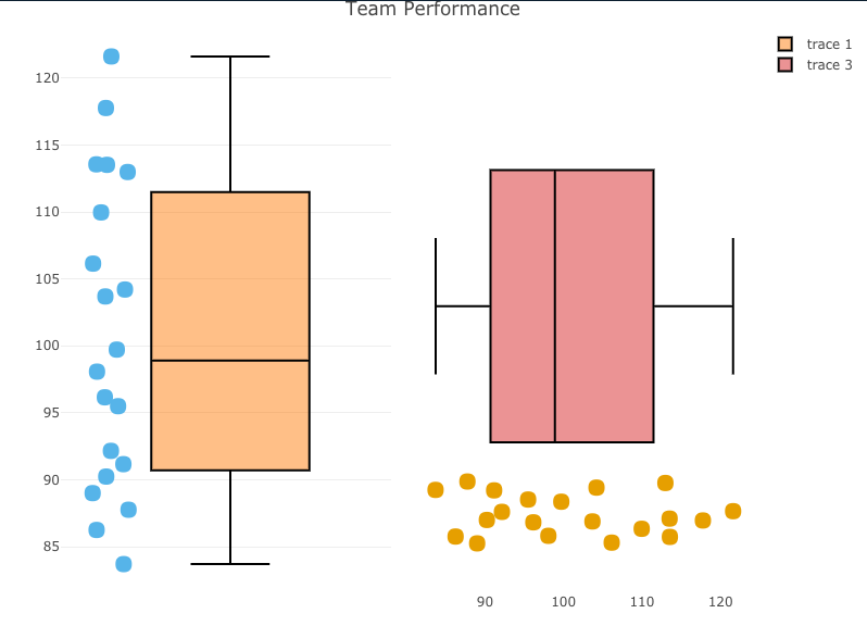
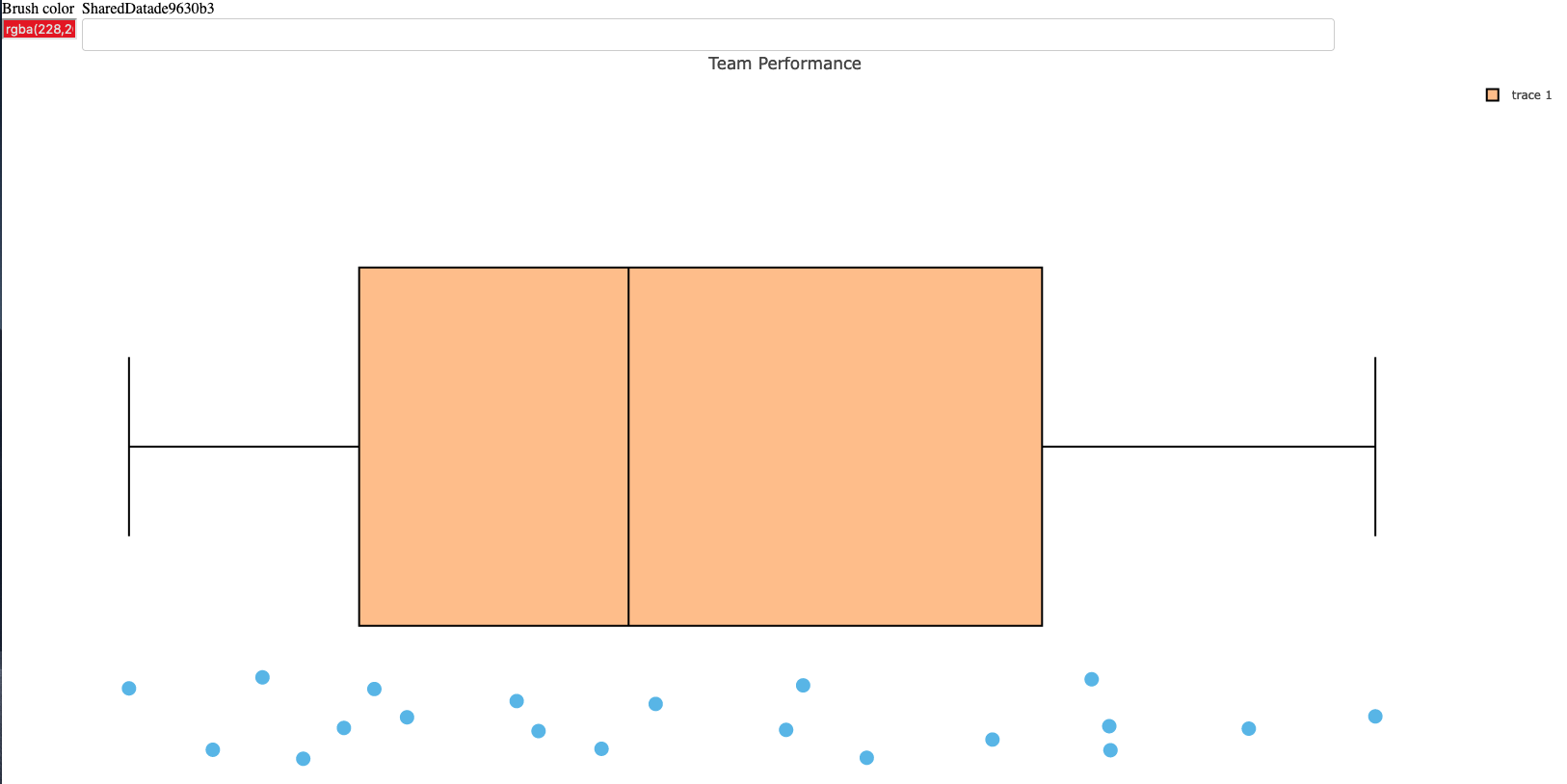
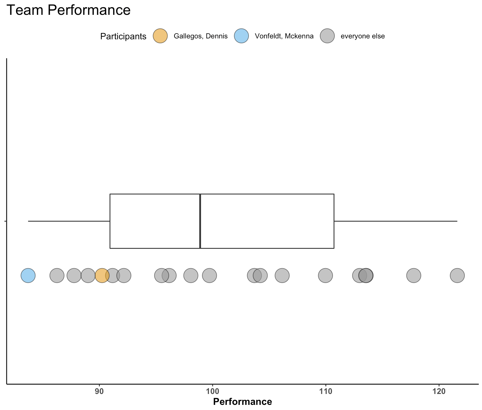
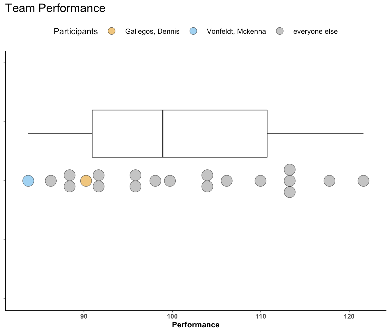
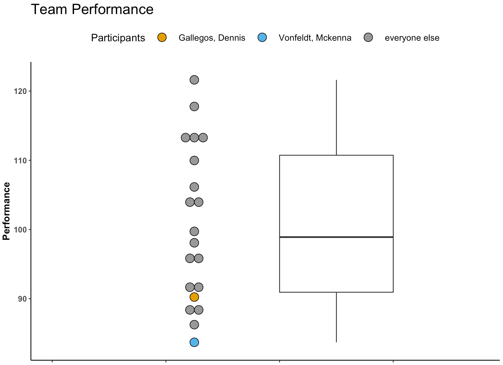
Given these different options, I figured I’d throw together a quick article to show what they look like and how to calculate them in R. The discussion is right in line with the last 2 blog articles about using boxplots and dotplots to visualize athlete testing data (Part 1 and Part 2).
Simulate Data
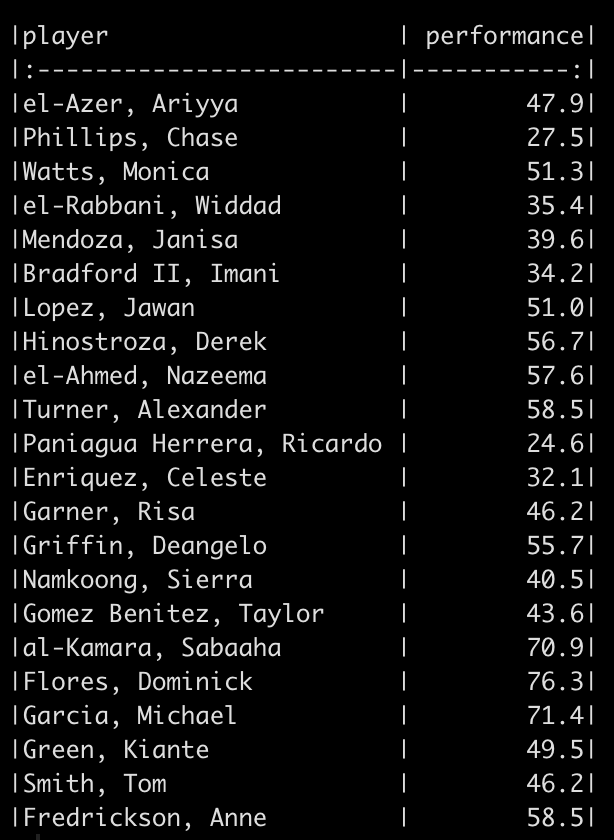
We will simulate performance test results for 22 different athletes. To do this, we take advantage of the rnorm() function in R and draw from 3 different normal distributions to produce 20 tests results. Since I used set.seed() you will be able to reproduce my results exactly. After creating 20 simulations I added 2 additional athletes to the data set and gave them test scores that were exactly the same as two other athletes in the data so that we had some athletes with the same performance outcome.

Percentile Rank
The percentile rank reflects the percentage of observations that are below a certain score. This value is displayed in 100 theoretical divisions of the observed data. Thus, the top score in the data represents 100 and every value falls below that.
To calculate the percentile rank we simply rank the observed performance values and then divide by the number of observations.
Let’s start by sorting the performance scores so that they are in order from lowest to highest.

Next, we rank these values.

Notice that when we sort the data we see that the values 58.5 and 46.2 are repeated twice. Once we rank them we see that the rank values are also correctly repeated. We can get rid of the half points for these repeated observation by using the trunc() function, which will truncate the values.

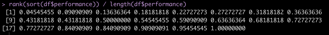
Finally, to get the percentile rank, we divide by the total number of observations.

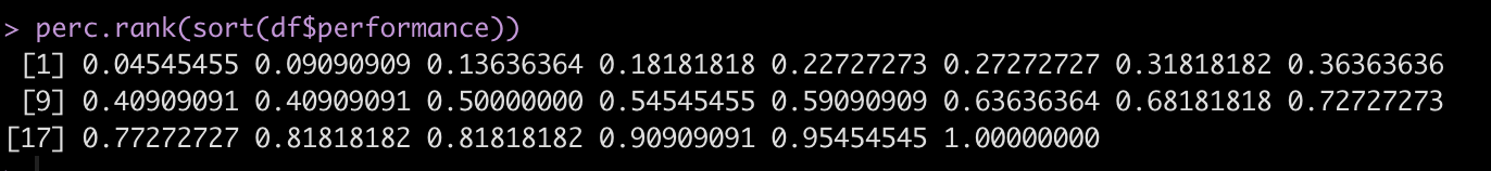
Instead of always having to walk through these steps, we can create a function to do the steps for us in one line of code. This will come in handy when we compare all of these methods later on.
perc.rank <- function(x){
  trunc(rank(x))/length(x)
}

perc.rank(sort(df$performance))

Percentiles
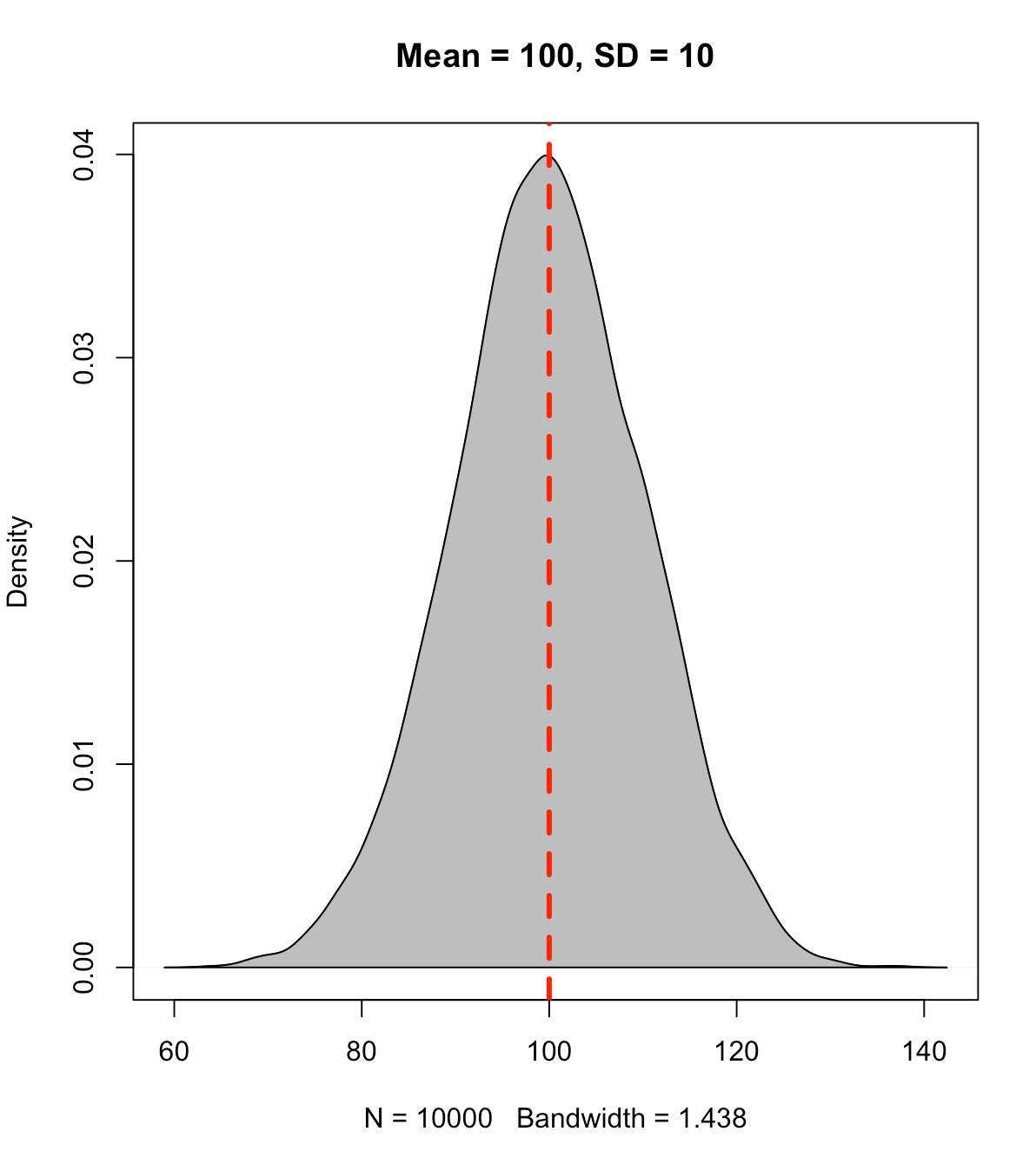
A percentile value is different than a percentile rank in that the percentile value reflects the observed score relative to a population mean and standard deviation. Often, this type of value has been used to represent how well a student has performed on a standardized test (e.g., SAT, ACT, GRE, etc.). The percentile value tells us the density of values below our observation. Thus, the percentile value represents a cumulative distribution under the normal curve, below the point of interest. For example, let’s say we have a bunch of normally distributed data with a mean of 100 and standard deviation of 10. If we plot the distribution of the data and drop a line at 100 (the mean), 50% of the data will fall below and it 50% above it.
set.seed(1)
y <- rnorm(n = 10000, mean = 100, sd = 10)

plot(density(y), col = 'black',
  main = 'Mean = 100, SD = 10')
polygon(density(y), col = 'grey')
abline(v = 100, col = 'red', lty = 2, lwd = 3)

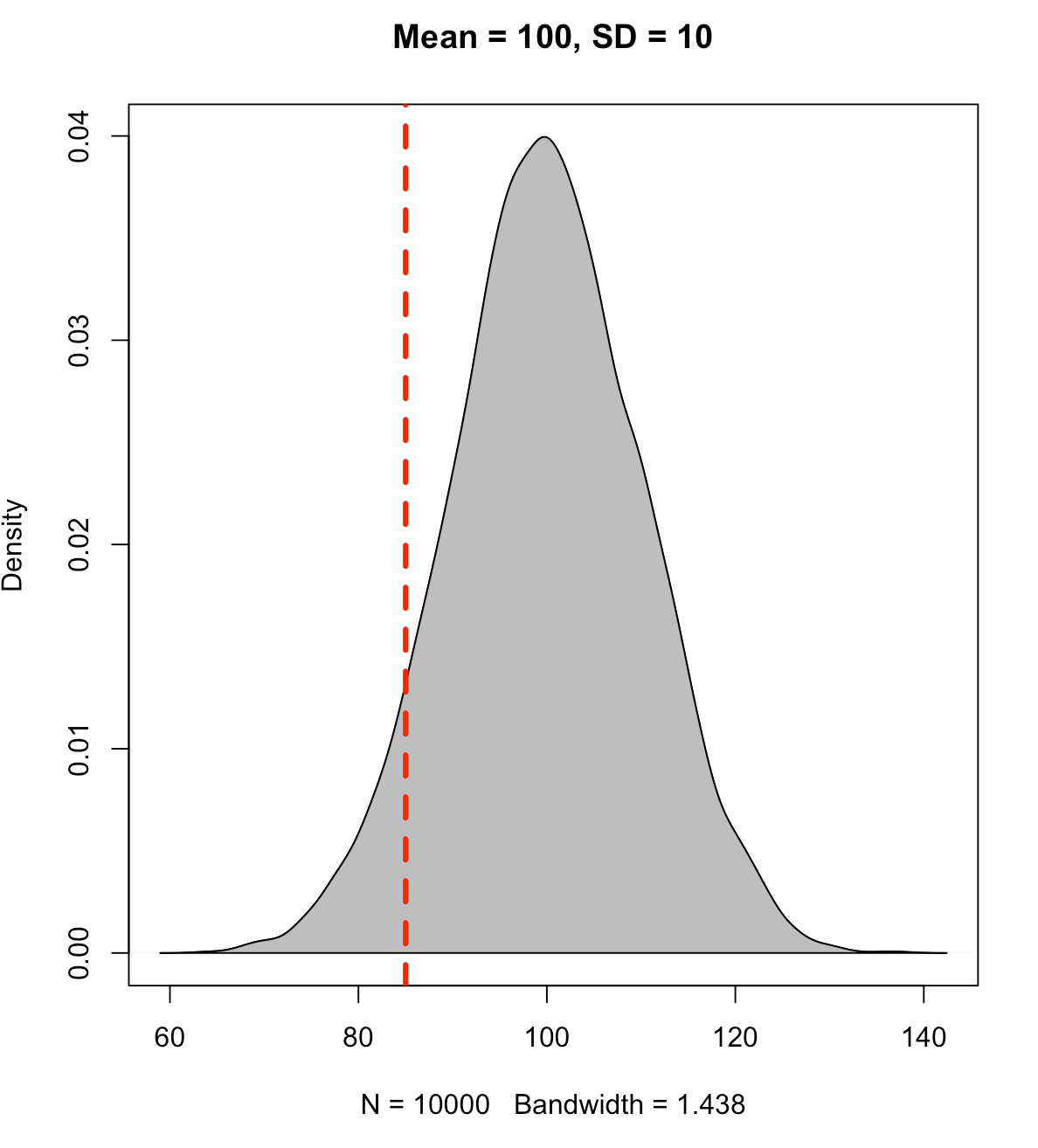
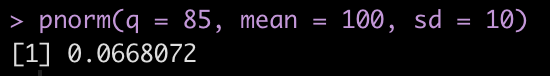
Instead, if we place the line at an observation of 85 we will see that approximately 7% of the data falls below this point (conversely, 93% of the data is above it).

To find the cumulative distribution below a specific observation we can use the pnorm() function and pass it the observation of interest, the population mean, and the standard deviation.
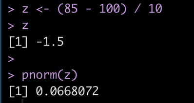
Alternatively, we can obtain the same value by first calculating the z-score of the point of interest and simply passing that into the pnorm() function.
z = (observation – mean) / sd
We find that the z-score for 85 is -1.5 standard deviations below the mean.
We will write a z-score function to use later on.
z_score <- function(x, avg, SD){
  z = (x - avg) / SD
  return(z)
}
T-score
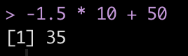
As we saw above, the score of 85 led to a z-score of -1.5. Sometimes having the data scaled to a mean of 0 with values above and below it can difficult for decision-makers to interpret. As such, we can take the z-score and turn it into a a t-score, ranging from 0-100, where 50 represents average, 40 and 60 represent ± 1 standard deviation, 30 and 70 represent ± 2 standard deviation, and 20 and 80 represent ± 3 standard deviations from the mean.
t = observation*10 + 50
Therefore, using the z-score value of -1.5 we end up with a t-score of 35.
We will make a t-score function to use on our athlete simulated data.
t_score <- function(z){
  t = z * 10 + 50
  return(t)
}
Returning to the athlete simulated data
We now return to our athlete simulated data and apply all of these approaches to the performance data. For the z-score, t-score, and percentile values, I’ll start by using the mean and standard deviation of the observed data we have.
df_ranks_v1 <- df %>%
mutate(percentile_rank = perc.rank(performance),
percentile_value = pnorm(performance, mean = mean(performance), sd = sd(performance)),
z = z_score(x = performance, avg = mean(performance), SD = sd(performance)),
t = t_score(z)) %>%
mutate(across(.cols = percentile_rank:t,
~round(.x, 2)))
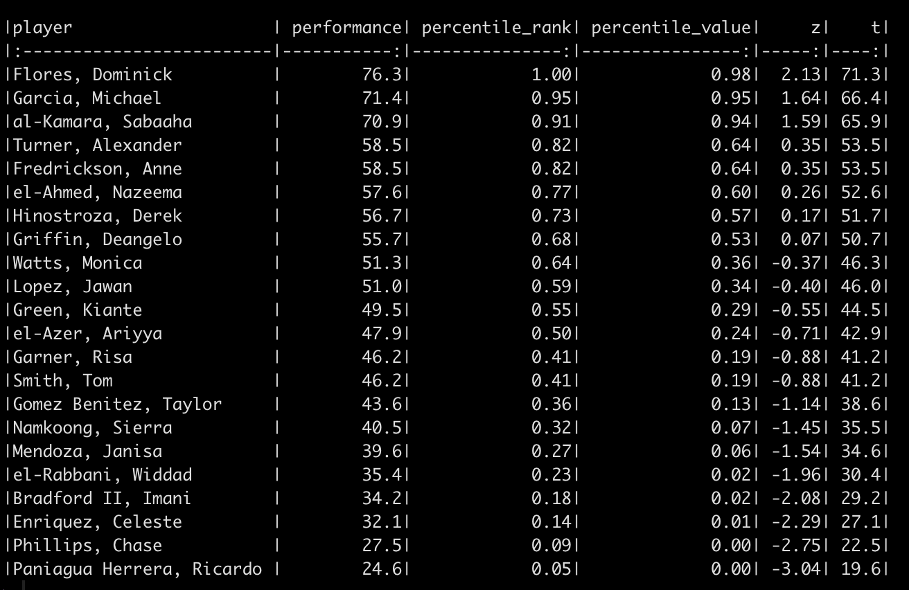
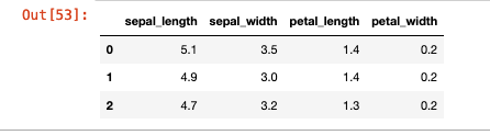
df_ranks_v1 %>%
arrange(desc(percentile_rank)) %>%
knitr::kable()
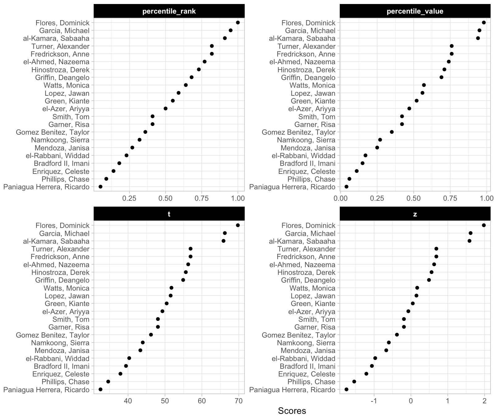
We can also plot these values to provide ourselves a visual to compare them.

We can see that the order of the athletes doesn’t change based on the method. This makes sense given that the best score for this group of athletes is always going to be the best score and the worst will always be the worst. We do see that the percentile rank approach assigns the top performance as 100%; however, the percentile value assigns the top performance a score of 98%. This is because the percent value is based on the parameters of the normal distribution (mean and standard deviation) and doesn’t rank the observations from best to worse as the percentile rank does. Similarly, the other two scores (z-score and t-score) also use the distribution parameters and thus follow the same pattern as the percentile value.
Why does this matter? The original discussion was about athletes within a given season, on one team. If all we care about is the performance of that group of athletes, on that team, in that given season, then maybe it doesn’t matter which approach we use. However, what if we want to compare the group of athletes to previous teams that we’ve had or to a population mean and standard deviation that we’ve obtained from the league (or from scientific literature)? In this instance, the percentile rank value will remain unchanged but it will end up looking different than the other three scores because it doesn’t depend on the mean and standard deviation of the population.
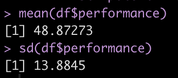
For example, the mean and standard deviation of our current team is 48.9 ± 13.9.
Perhaps our team is currently below average for what we expect from the population. Let’s assume that the population we want to compare our team to has a mean and standard of 55 ± 10.
df_ranks_v2 <- df %>%
  mutate(percentile_rank = perc.rank(performance),
         percentile_value = pnorm(performance, mean = 55, sd = 10),
         z = z_score(x = performance, avg = 55, SD = 10),
         t = t_score(z)) %>%
  mutate(across(.cols = percentile_rank:t,
                ~round(.x, 2)))

df_ranks_v2 %>%
  arrange(desc(percentile_rank)) %>%
  knitr::kable()

Again, the order of the athletes’ performance doesn’t change and thus the percentile rank of the athletes also doesn’t change. However, the percentile values, z-scores, and t-scores now tell a different story. For example, el-Azer, Ariyya scored 47.9 which has a percentile rank of 50% for the observed performance scores of this specific team. However, this value relative to our population of interest produces a z-score of -0.71, a t-score of 42.9, and a percentile value indicating that only 24% of those in the population who are taking this test are below this point. The athlete looks to be average for the team but when compared to the population they look to be below average.
Wrapping Up
There are a number of ways to display the outcomes on a test for athletes. Using percentile rank, we are looking specifically at the observations of the group that took the given test. If we use percentile value, z-scores, and t-scores, we are using properties of the normal distribution and, often comparing the observed performance to some known population norms. There probably isn’t a right or wrong approach here. Rather, it comes down to the type of story you are looking to tell with your data.
The full code for this article is available on my GITHUB page.