Category Archives: R Tips & Tricks

Weakley et al. (2022). Velocity-Based Training: From Theory to Application – R Workbook

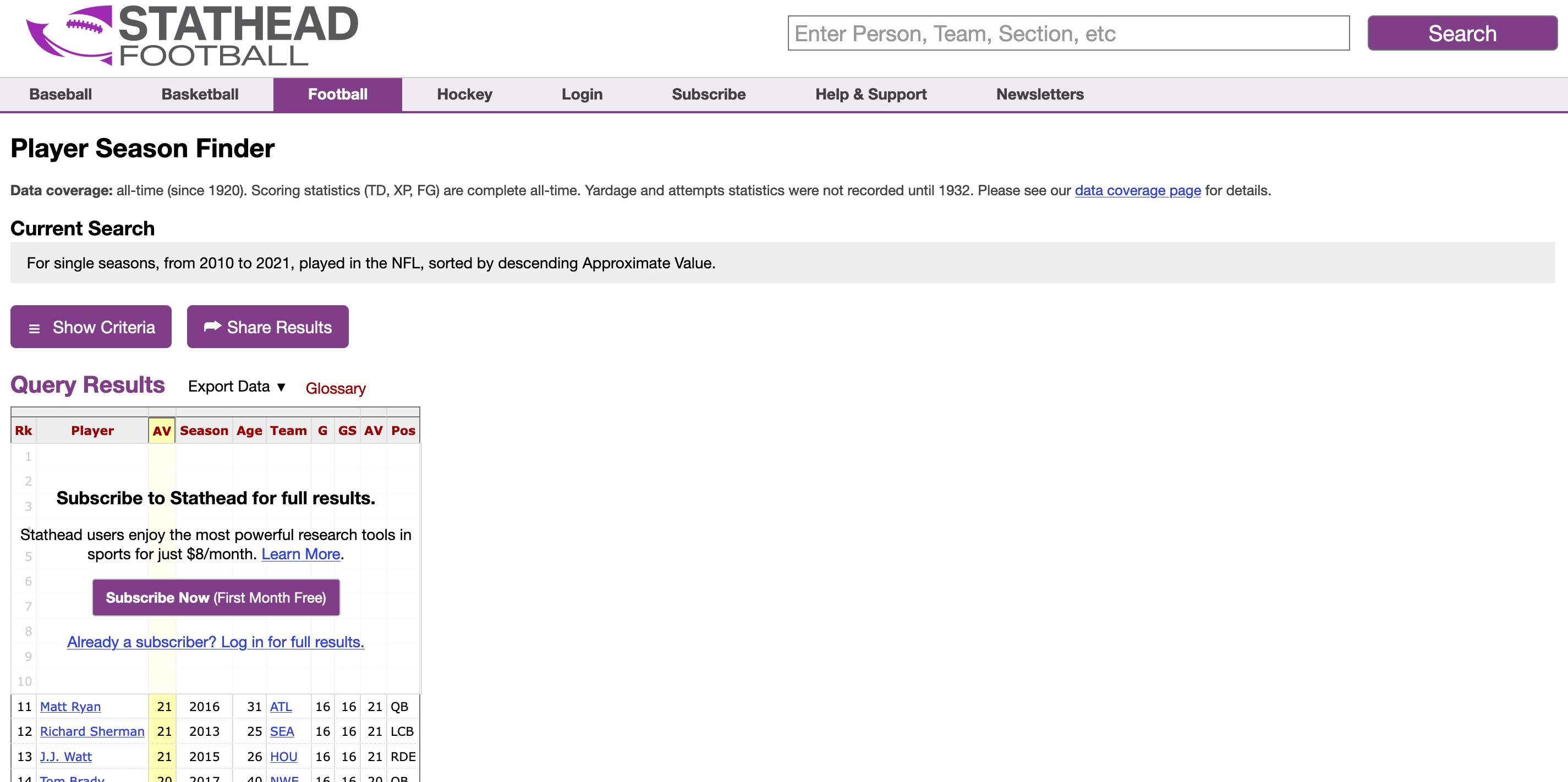
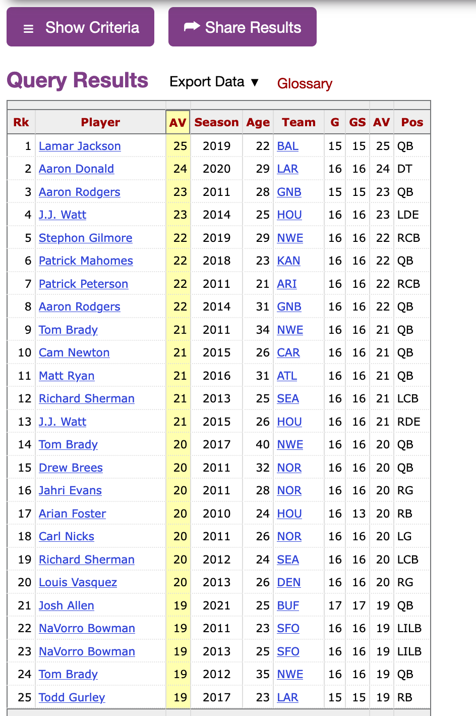
Velocity-based training (VBT) is a method employed by strength coaches to prescribe training intensity and volume based off of an individual athlete’s load-velocity profiles. I discussed VBT last year when I used {shiny} to build an interactive web application for visualizing and comparing athlete outputs.

Specific to this topic, I recently read the following publication: Weakley, Mann, Banyard, McLaren, Scott, and Garcia-Ramos. (2022). Velocity-based training: From theory to application. Strength Cond J; 43(2): 31-49.

The paper aimed to provide some solutions for analyzing, visualizing, and presenting feedback around training prescription and performance improvement when using VBT. I enjoyed the paper and decided to write an R Markdown file to provide code that can accompany it and (hopefully) assist strength coaches in applying some of the concepts in practice. I’ll summarize some notes and thoughts below, but if you’d like to read the full R Markdown file that explains and codes all of the approaches in the paper, CLICK HERE>> Weakley–2021—-Velocity-Based-Training—From-Theory-to-Application—Strength-Cond-J.

If you’d like the CODE and DATA to run the analysis yourself, they are available on my GitHub page.

Paper/R Markdown Overview

Technical Note: I don’t have the actual data from the paper. Therefore, I took a screen shot of Figure 3 in the text and used an open source web application for extracting data from figures in research papers. This requires me to go through and manually click on the points of the plot itself. Consequently, I’m not 100% perfect, so there may be subtle differences in my data set compared to what was used for the paper.

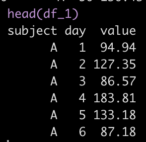
The data used in the paper reflect 17-weeks of mean concentric velocity (MCV) in the 100-kg back squat for a competitive powerlifter, tested once a week. The two main figures, which, along with the analysis, I will recreate are Figure 3 and Figure 5.

Figure 3 is a time series visual of the athlete while Figure 5 provides an analysis and visual for the athlete’s change across the weeks in the training phase.

Figure 3

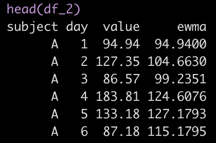
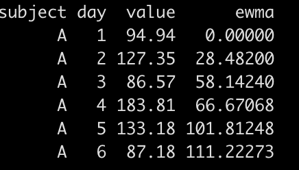
The first 10-weeks represent the maintenance phase for the athlete, which was followed by a 7-week training phase. The maintenance phase sessions were used to build a linear regression model which was then used to visualize the athlete’s change over time along with corresponding confidence interval around each MCV observation. The model output looks like this:

The standard (typical) error was used to calculate confidence intervals around the observations. To calculate the standard error, the authors’ recommend one of two approaches:

1) If you have group-based test-retest data, they recommend taking the difference between the test-retest outcomes and calculating the standard error as follows:

  • SE.group = sd(differences) / sqrt(2)

2) If you have individual observations, they recommend calculating the standard error like this:

  • SE.individual = sqrt(sum.squared.residuals) / (n2))

Since we have individual athlete data, we will use the second option, along with the t-critical value for 80% CI, to produce Figure 3 from the paper :

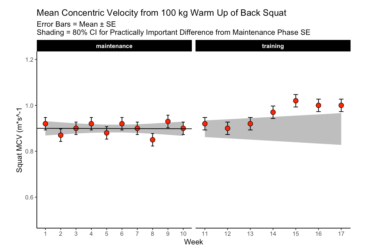
The plot provides a nice visual of the athlete over time. We see that, because the linear model is calculated for the maintenance phase, as time goes on, the shaded standard error region gets wider. The confidence intervals around each point estimate are there to encourage us to think past just a point estimate and recognize that there is some uncertainty in every test outcome that cannot be captured in a single value.

Figure 5

This figure visualizes the change in squat velocity for the powerlifter in weeks 11-17 (the training phase) relative to the mean squat velocity form the maintenance phase, representing the athlete’s baseline performance.

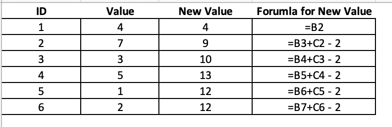
Producing this plot requires five pieces of information:

  1. Baseline average for the maintenance phase
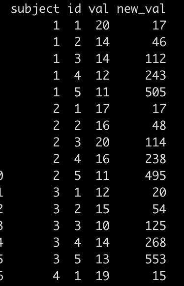
  2. The difference between the observed MVC in each training week and the maintenance average
  3. Calculate the t-critical value for the 90% CI
  4. Calculate the Lower 90% CI
  5. Calculate the Upper 90% CI

Obtaining this information allows us to produce the following table of results and figure:

Are the changes meaningful?

One thing the authors’ mention in the paper are some approaches to evaluating whether the observed changes are meaningful. They recommend using either equivalence tests or second generation p-values. However, they don’t go into calculating such things on their data. I honestly am not familiar with the latter option, so I’ll instead create an example of using an equivalence test for the data and show how we can color the points within the plot to represent their meaningfulness.

Equivalence testing has been discussed by Daniel Lakens and colleagues in their tutorial paper, Lakens, D., Scheel, AM., Isager, PM. (2018). Equivalence testing for psychological reserach: A tutorial. Advances in Methods and Practices in Psychological Science. 2018; 1(2): 259-269.

Briefly, equivalence testing uses one-sided t-tests to evaluate whether the observed effect is larger or smaller than a pre-specified range of values surrounding the effect of interest, termed the smallest effect size of interest (SESOI).

In our above plot, we can consider the shaded range of values around 0 (-0.03 to 0.03, NOTE: The value 0.03 was provided in the text as the meaningful change for this athlete to see an ~1% increase in his 1-RM max) as the region where an observed effect would not be deemed interesting. Outside of those ranges is a change in performance that we would be most interested in. In addition to being outside of the SESOI region, the observed effect should be substantially large enough relative to the standard error around each point, which we calculated from our regression model earlier.

Putting all of this together, we obtain a the same figure above but now with the points colored specific to the p-value provided from our equivalence test:

Warpping Up

Again, if you’d like the full markdown file with code (click the ‘code’ button to display each code chunk) CLICK HERE >> Weakley–2021—-Velocity-Based-Training—From-Theory-to-Application—Strength-Cond-J

There are always a number of ways that analysis can unfold and provide valuable insights and this paper reflects just one approach. As with most things, I’m left with more questions than answers.

For example, Figure 3, I’m not sure if linear regression is the best approach. As we can see, the grey shaded region increases in width overtime because time is on the x-axis (independent variable) and the model was built on a small portion (the first 10-weeks) of the data. As such, with every subsequent week, uncertainty gets larger. How long would one continue to use the baseline model? At some point, the grey shaded region would be so wide that it would probably be useless. Are we too believe that the baseline model is truly representative of the athlete’s baseline? What if the baseline phase contained some amount of trend — how would the model then be used to quantify whatever takes place in the training phase? Maybe training isn’t linear? Maybe there is other conditional information that could be used?

In Figure 5, I wonder about the equivalence testing used in this single observation approach. I’ve generally thought of equivalence testing as a method comparing groups to determine if the effect from an intervention in one group is larger or smaller than the SESOI. Can it really work in an example like this, for an individual? I’m not sure. I need to think about it a bit. Maybe there is a different way such an analysis could be conceptualized? A lot of these issues come back to the problem of defining the baseline or some group of comparative observations that we are checking our most recent observation against.

My ponderings aside, I enjoyed the paper and the attempt to provide practitioners with some methods for delivering feedback when using VBT.

Web Scraping Webpages that Require Login info

Someone recently asked me how to go about web scraping a webpage that requires you to login. The issue with these types of situations is that the URL you are scraping wont allow you to access the data, even if you are signed into the website. The solution is that within R you actually need to set up your login info prior to scraping from the desired URL.

Let’s take a simple example. Here is the player Approximate Value page from Pro-Football-Reference:

URL

Notice that the first 10 rows are not accessible to us because they are part of a subscription service. Also, if we were to navigate to the URL (as opposed to looking at my small screen shot), you’ll see only 20 rows of data, when the actual page (once logged in) has 200 rows!

Once I log into the account I can see all of the hidden info:

Let’s start by seeing what happens when I scrape this page, now that I’m logged in


ACK!! It didn’t work. Even though I’m logged into the website, R doesn’t know it. It just reads the URL as is and thus only returns 20 rows of data with 10 of the rows being blank, since they are covered up on the website.

Solving the Problem

The way we will solve this problem is to get the URL for the login page and pass it to the session() function in R:


Once you’ve loaded up the login page then you need to get a login form and fill it out with your username and password, like this:

Technical Note: The last step where you are changing the info in field 4 to “button” is required, otherwise you will get an error in the next step. I’m not entirely sure why it is required and after failing a few times and then doing some googling, I’ve found this to be an easy enough solution.

Once you have filled out the login form, you simply submit it to the website with the session_submit() function and then repeat the web scraping process that we did at the beginning, however instead of using the read_html() function to pass the URL you will use the session_jump_to() function and provide it with the info about the login page and the URL you are scraping:


Now, all the data on that page will be available to you:

Happy scraping!!


Tidymodels model fitting template

We recently completed a 10 episode series on the Tidy Explained screen cast about building models within the {tidymodels} framework of R.

To tie it the series together I put together an RMarkdown file that walks through the model fitting process in {tidymodels}. The RMarkdown template provides a step-by-step process that one can take when building {tidymodels} on their own data.

If you knit the RMarkdown template, you will get an html report that covers the basics of:

  • Splitting data into training, testing, and cross validation sets
  • Specifying models
  • Pre-processing with model recipes
  • Setting up workflows and workflowsets
  • Fitting models and parameter tuning
  • Evaluating model outputs
  • Making predictions on test data
  • Saving the model workflow for future model deployment
  • Loading the saved model workflow and deploying it on a new data set

To access the template, go to my GITHUB page.

Below are the 10 {tidymodels} episodes we did on Tidy Explained if you’d like to see the processes performed in real time:

TidyX 77: Intro to tidymodels
TidyX 78: Splits & Recipes
TidyX 79: Cross-Validation & Model Metrics
TidyX 80: Tuning Decision Trees
TidyX 81: Logistic Regression
TidyX 82: Random Forest Classifier
TidyX 83: Naive Bayes Classifier
TidyX 84: Workflowsets
TidyX 85: Workflowsets & Parameter Tuning
TIdyX 86: Tidymodels interview with Julia Silge

R Tips & Tricks: Excel Within Column Iteration in R (part 2)

Earlier this week I shared a method for doing within column iteration in R, as you might do in excel. For example, you want to create a new column that requires a starting value from a different column (or a 0 value) and then requires new values within that column to iterate over the prior values. The way I handled this was to use the accumuate() function available in the {tidyverse} package.

The article got some good feedback and discussion on Twitter. For example, Thomas Mock, provided some examples of using the {slider} package to handle window functions, see HERE and HERE. The package looks to be very handy and easy to use. I’m going have to play around with it some more.

Someone else asked, “how might we do this in a for() loop?”

It’s a good question. Sometimes you might need to use base R or sometimes the for() loop might be easier. So, let’s walk through an example:

Simulate Data

First, we need to simulate a basic data set:

library(tidyverse)

df <- tibble(
  id = 1:5,
  val = c(5,7,3,4,2)
)

df

Setting Up the Problem

Let’s say we want to create a new value that applies a very simple algorithm:

New Value = observed + 2 * lag(new value)

Putting the above data in excel the formula and answer looks like this:

Notice that the first new value starts with our initial observation (5) and then begins to iterate from there.

Writing the for() loop

for() loops can sometimes be scary but if you sequentially think through what you are trying to do you can often come up with a reasonable solution. Let’s step through this one:

  1.  We begin outside of the for() loop by creating two elements. We create N which simply gives us a count of the number of observations in our val column and we create new_val which is nothing more than a place holder for the new values we will create. Notice that the new_val place holder starts with the first element of the df$val column because, remember, we need to begin the new column with our first value observation in the val column. After that, I simply concatenate a bunch of NA values that will be populated with the new values that the for() loop will produce. Notice that I have NA repeat for N-1 times. This is important, as represents the number of observations in the val column and since we’ve already put a place holder in for the first observation we need to remove one of the NA’s to ensure the new_val column will be the same length as the val column.
  2. Next, we create our loop. I specify that I want to iterate over all “i” iterations from 2 to N. Why 2? Because the first value is already specified, as discussed above. Inside the for() loop, for each iteration that the loop runs it will store the new value, “i” in the new_val vector we created above. The equation that we specified earlier is within the for loop and I use “i” to index the observations. For example, for the second observation, what the for() loop is doing is saying, df$val[2] + new_val[2 – 1]*2, and for the third time through the loop it says, df$val[3] + new_val[3 – 1]*2, etc. until it goes through all N observations. Everything in the brackets is simply specifying the row indexes.
## We want to create a new value
# New Value = observed + 2 * lag(new value)
# The first value for the new value is the first observation in row one for value

N <- length(df$val)
new_val <- c(df$val[1], rep(NA, N-1))

for(i in 2:N){

  new_val[i] <- df$val[i] + new_val[i - 1]*2
  
}


Once the loop is done running we can simply attach the results to our data frame and see what it looks like:

Same results as the excel sheet!

Wrapping this into a function

After seeing how the for() loop works, you might want to wrap it up into a function so that you don’t need to do the first steps of creating an element for the number of iterations and vector place holder. Also, having it in a function might be useful if you need to frequently use it for other data sets.

We simply wrap all of the steps into a single function that takes an input of the data frame name and the value column that has your most recent observations. Run the function on the data set above and you will obtain the same output.

iterate_column_func <- function(df, val){
  
  N <- length(df$val)
  new_val <- c(df$val[1], rep(NA, N-1))
  
  for(i in 2:N){
    
    new_val[i] <- df$val[i] + new_val[i - 1]*2
    
  }
  
  df$new_val <- new_val
  return(df)
}

iterate_column_func(df, val)


Applying the function to multiple subjects

What if we have more than one subject that we need to apply the function to?

First, we simulate some more data:

df_2 <- tibble(
  subject = as.factor(rep(1:10, each = 5)),
  id = rep(1:5, times = 10),
  val = round(runif(n = 50, min = 10, max = 20), 0)
)

df_2

Next, I’m going to make a slight tweak to the function. I’m going to have the output get returned as a single column data frame.

iterate_column_func <- function(x){
  
  N <- length(x)
  new_val <- c(x[1], rep(NA, N-1))
  
  for(i in 2:N){
    
    new_val[i] <- x[i] + new_val[i - 1]*2
    
  }
  
  new_val <- as.data.frame(new_val)
  return(new_val)
}

Now, I’m going to apply the custom function to my new data frame, with multiple subjects, using the group_modify() function in {tidyverse}. This function allows us to apply other functions to groups of subjects, iterating over them and producing a data frame as a result.


new_df <- df_2 %>%
  group_by(subject) %>% 
  group_modify(~iterate_column_func(.x$val)) %>%
  ungroup()

Then, I simply bind this new data to the original data frame and we have our new_val produced within individual.

df_2 %>%
  bind_cols(new_df %>% select(-subject)) %>% as.data.frame()

Conclusion

And there you go, within column iteration in R, just as you would do in excel. Part 1 covered an approach in {tidyverse} while Part 2 used for() loops in base R to accomplish the same task.

The full code for this article is available on my GitHub page.

R Tips & Tricks: Recreating within column iteration as you would do in excel

One of the easiest things to do in excel is within column iteration. What I mean by this is you create a new column where the starting value is a 0 or a value that occurs in a different column and then all of the following values within that column depend on the value preceding it.

For example, in the below table we can see that we have a value for each corresponding ID. The New Value is calculated as the most recent observation of Value + lag(New Value) – 2. This is true for all observations except the first observation, which simply takes Value of the first ID observation. So, in ID 2, we get: New Value = 7 + 4 – 2 = 9 and in ID 3 we get: New Value = 3 + 9 – 2 = 10.


This type of function is pretty common in excel but it can be a little tricky in R. I’ve been meaning to do a blog about this after a few questions that I’ve gotten and Aaron Pearson reminded me about it last night, so let’s try and tackle it.

Creating Data

We will create two fake data sets:

  • Data set 1 will be a larger data set with multiple subjects.
  • Data set 2 will only be one subject, a smaller data set for us to first get an understanding of what we are doing before trying to perform the function over multiple people.


library(tidyverse)

## simulate data
set.seed(1)
subject <- rep(LETTERS[1:3], each = 50)
day <- rep(1:50, times = 3)
value <- c(
  round(rnorm(n = 20, mean = 120, sd = 40), 2),
  round(rnorm(n = 10, mean = 150, sd = 20), 2),
  round(rnorm(n = 20, mean = 110, sd = 30), 2),
  round(rnorm(n = 20, mean = 120, sd = 40), 2),
  round(rnorm(n = 10, mean = 150, sd = 20), 2),
  round(rnorm(n = 20, mean = 110, sd = 30), 2),
  round(rnorm(n = 20, mean = 120, sd = 40), 2),
  round(rnorm(n = 10, mean = 150, sd = 20), 2),
  round(rnorm(n = 20, mean = 110, sd = 30), 2))

df_1 <- data.frame(subject, day, value) df_1 %>% head()

### Create a data frame of one subject for a simple example
df_2 <- df_1 %>%
  filter(subject == "A")

Exponentially Weighted Moving Average (EWMA)

We will apply an exponentially weighted moving average to the data as this type of equation requires within column aggregation.

EWMA is calculated as:

EWMA_t = lamda*x_t + (1 – lamda) * Z_t-1

Where:

  • EWMA_t = the exponentially weighted moving average value at time t
  • Lamda = the weighting factor
  • x_t = the most recent observation
  • Z_t-1 = the lag of the EWMA value

accumulate()

Within {tidyverse} we will use the accumulate() function, which allows us to create this type of within column aggregation. The function takes a few key arguments:

  • First we need to pass the function the name of the column of data with our observations over time
  • .y which represents the value of our most recent observation
  • .f which is the function that we want to apply to our within column aggregation (in this example we will use the EWMA equation)
  • .x which is going to provide us with the lagged value within the new column we are creating

Here is what it looks like in our smaller data set, df_2


df_2 <- df_2 %>%
  mutate(ewma = accumulate(value, ~ lamda * .y + (1 - lamda) * .x))

Here, we are using mutate() to create a new column called ewma. We used accumulate() and passed it the value column, which is the column of our data that has our observations and our function for calculating ewma, which follows the tilde.

Within this function we see .y, the most recent observation and .x, the lag ewma value. By default, the first row of the new ewma column will be the first observation in the value row. Here is what the first few rows of the data look like:

Now that new column has been created we can visualize the observed values and the EWMA values:

Applying the approach to all of the subjects

To apply this approach to all of the subjects in our data we simply need to use the group_by() function to tell R that we want to have the algorithm start over whenever it encounters a new subject ID.


df_1 <- df_1 %>%
  group_by(subject) %>%
  mutate(ewma = accumulate(value, ~ lamda * .y + (1 - lamda) * .x))

And then we can plot the outcome:

Pretty easy!

What if we want the start value to be 0 (or something else) instead of the first observation?

This is a quick fix within the accumulate() function by using the .init argument and simply passing it whatever value you want the new column to begin with. What you need to be aware of when you do this, however, is that this argument will add an additional observation to the vector of data and thus we need to remove the last row of the data set to ensure that {tidyverse} can perform the operation without giving you an error. To accomplish this, when I pass the value column to the function I add a bracket and then minus 1 of the total count, n(), of observations in that column.

df_2 %>%
  mutate(ewma = accumulate(value[-n()], ~ lamda * .y + (1 - lamda) * .x, .init = 0)) %>%
  head()

Now we see that the first value in ewma is 0 instead of 94.94, which of course changes all of the values following it since the equation is using the lagged ewma value (.x).

For the complete code, please see my GitHub Page.