Category Archives: R Tips & Tricks

Deriving a Confidence Interval from an Estimate and a p-value

Although most journals require authors to include confidence intervals into their papers it isn’t mandatory for all journal (merely a recommendation). Additionally, there may be occasions when you are reading an older paper from a time when this mandate/recommendation was not enforced. Finally, sometimes abstracts (due to word count limits) might only present p-values and estimates, in which case you might want to quickly obtain the confidence intervals to help organize your thoughts prior to diving into the paper. In these instances, you might be curious as to how you can get a confidence interval around the observed effect when all you have is a p-value.

Bland & Altman wrote a short piece of deriving confidence interval from only an estimate and a p-value in a 2011 paper in the British Medical Journal:

Altman, DG. Bland, JM. (2011). How to obtain the confidence interval from a p-value. BMJ, 343: 1-2.

Before going through the approach, it is important to note that they indicate a limitation of this approach is that it wont be as accurate in smaller samples, but the method can work well in larger studies (~60 subjects or more).

The Steps

The authors’ list 3 easy steps to derive the confidence interval from an estimate and p-value:

  1. Calculate the test statistic for a normal distribution from the p-value.
  2. Calculate the standard error (ignogre the minus sign).
  3. Calculate the 95% CI using the standard error and a z-critical value for the desired level of confidence.
  4. When doing this approach for a ratio (e.g., Risk Ratio, Odds Ratio, Hazard Ratio), the formulas should be used with the estimate on the log scale (if it already isn’t) and then exponentiate (antilog) the confidence intervals to put the results back to the normal scale.

Calculating the test statistic

To calculate the test statistic use the following formula:

z = -0.862 + sqrt(0.743 – 2.404 * log(p.value))

Calculating the standard error

To calculate the standard error use the following formula (remember that we are ignoring the sign of the estimate):

se = abs(estimate) / z

If we are dealing with a ratio, make sure that you are working on the log scale:

se = abs(log(estimate)) / z

Calculating the 95% Confidence Limits

Once you have the standard error, the 95% Confidence Limits can be calculated by multiplying the standard error by the z-critical value of 1.96:

CL.95 = 1.96 * se

From there, the 95% Confidence Interval can be calculated:

low95 = Estimate – CL.95
high95 = Estimate + CL.95

Remember, if you are working with rate statistics and you want to get the confidence interval on the natural scale, you will need to take the antilog:

low95 = exp(Estimate – CL.95)
high95 = exp(Estimate + CL.95)


Writing a function

To make this simple, I’ll write everything into a function. The function will take three arguments, which you will need to obtain from the paper:

  1. p-value
  2. The estimate (e.g., difference in means, risk ratio, odds ratio, hazard ratio, etc)

The function will default to log = FALSE but if you are working with a rate statistic you can change the argument to log = TRUE to get the results on both the log and natural scales. The function also takes a sig_digits argument, which defaults to 3 but can be changed depending on how many significant digits you need.

estimate_ci_95 <- function(p_value, estimate, log = FALSE, sig_digits = 3){
  
  if(log == FALSE){
    
    z <- -0.862 + sqrt(0.743 - 2.404 * log(p_value))
    z

    se <- abs(estimate) / z
    se
    
    cl <- 1.96 * se
    
    low95 <- estimate - cl
    high95 <- estimate + cl
    
    list('Standard Error' = round(se, sig_digits),
         '95% CL' = round(cl, sig_digits),
         '95% CI' = paste(round(low95, sig_digits), round(high95, sig_digits), sep = ", "))
    
  } else {
    
    if(log == TRUE){
      
      z <- -0.862 + sqrt(0.743 - 2.404 * log(p_value))
      z
      
      se <- abs(estimate) / z
      se
      
      cl <- 1.96 * se
      
      low95_log_scale <- estimate - cl
      high95_log_scale <- estimate + cl
      
      low95_natural_scale <- exp(estimate - cl)
      high95_natural_scale <- exp(estimate + cl)
      
      list('Standard Error (log scale)' = round(se, sig_digits),
           '95% CL (log scale)' = round(cl, sig_digits),
           '95% CL (natural scale)' = round(exp(cl), sig_digits),
           '95% CI (log scale)' = paste(round(low95_log_scale, sig_digits), round(high95_log_scale, sig_digits), sep = ", "),
           '95% CI (natural scale)' = paste(round(low95_natural_scale, sig_digits), round(high95_natural_scale, sig_digits), sep = ", "))
      
    }
    
  }
  
}

 Test the function out

The paper provides two examples, one for a difference in means and the other for risk ratios.

Example 1

Example 1 states:

“the abstract of a report of a randomised trial included the statement that “more patients in the zinc group than in the control group recovered by two days (49% v 32%,P=0.032).” The difference in proportions was Est = 17 percentage points, but what is the 95% confidence interval (CI)?

estimate_ci_95(p_value = 0.032, estimate = 17, log = FALSE, sig_digits = 1)


Example 2

Example 2 states:

“the abstract of a report of a cohort study includes the statement that “In those with a [diastolic blood pressure] reading of 95-99 mm Hg the relative risk was 0.30 (P=0.034).” What is the confidence interval around 0.30?”

Here we change the argument to log = TRUE since this is a ratio statistic needs to be on the log scale.

estimate_ci_95(p_value = 0.034, estimate = log(0.3), log = TRUE, sig_digits = 2)

Try the approach out on a different data set to confirm the confidence intervals are calculated properly

Below, we build a simple logistic regression model for the PimaIndiansDiabetes data set from the {mlbench} package.

  • The odds ratios are already on the log scale so we set the argument log = TRUE to ensure we get results reported back to us on the natural scale, as well.
  • We use the summary() function to obtain the model estimates and p-values.
  • We use the confint() function to get the 95% Confidence Intervals from the model.
  • To get the confidence intervals on the natural scale we also take the exponent, exp(confint()).
  • We use our custom function, estimate_ci_95(), to see how well the results compare.
## get data
library(mlbench)
data("PimaIndiansDiabetes")
df <- PimaIndiansDiabetes

## turn outcome variable into a numeric (0 = negative for diabetes, 1 = positive for diabetes)
df$diabetes_num <- ifelse(df$diabetes == "pos", 1, 0)
head(df)

## simple model
diabetes_glm <- glm(diabetes_num ~ pregnant + glucose + insulin, data = df, family = "binomial")

## model summary
summary(diabetes_glm)


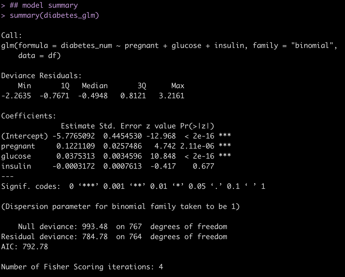
Calculate 95% CI from the p-values and odds ratio estimates.

Pregnant Coefficient

## 95% CI for the pregnant coefficient
estimate_ci_95(p_value = 2.11e-06, estimate = 0.122, log = TRUE, sig_digits = 3)


Glucose Coefficient

## 95% CI for the glucose coefficient
estimate_ci_95(p_value = 2e-16, estimate = 0.0375, log = TRUE, sig_digits = 3)


Insulin Coefficient

## 95% CI for the insulin coefficient
estimate_ci_95(p_value = 0.677, estimate = -0.0003, log = TRUE, sig_digits = 5)


Evaluate the results from the custom function to those calculated with the confint() function.

## Confidence Intervals on the Log Scale
confint(diabetes_glm)

## Confidence Intervals on the Natural Scale
exp(confint(diabetes_glm))

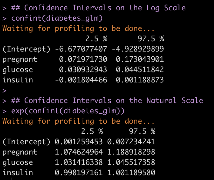
We get nearly the same results with a bit of rounding error!

Hopefully this function will be of use to some people as they read papers or abstracts.

You can find the complete code in a cleaned up markdown file on my GITHUB page.

Tyrese Maxey’s 3pt%, Bayes, Shrinkage

Some friends were discussing Philadelphia 76er’s point guard, Tyrese Maxey’s, three point% today. They were discussing how well he has performed over 72 games with a success rate of 43% behind the arc (at the time this data was scraped, 4/6/2022). While his percentage from 3pt range is very impressive I did notice that he has 294 attempts, which is less than 3 out of the 4 player’s that are ahead of him (Kyrie only has 214 attempts and he is ranked 3rd at the time of this writing) and Steph Curry is just behind Maxey in the ranking (42.4% success) with nearly 70 more attempts.

The question becomes, how can we be of Maxey’s three point percentage relative to those with more attempts? We will take a Bayesian approach, using a beta conjugate, to consider the success rate of these players relative to what we believe the average three point success rate is for an NBA shooter (our prior), which we will determine from observing 3 point shooting over previous 3 seasons.

NOTE: On basketball-reference.com, they have a nice check box that automatically will filter out players that are non-qualifiers for rate stats. After playing around with this, it appears that 200 attempts is their cut off. So, I will keep that and filter the data down to only those with 200 or more 3pt attempts.

All of the code, web scrapping, and csv files of the data (if you are looking to run it prior to when I scrapped it) are available on my GITHUB PAGE.

Exploratory Data Analysis

First, let’s view the top 10 three point shooters this season (size of the dot represents the number of three point attempts taken).

Visualize the distribution of three point attempts and three point% for the 2022 season, so far.

Establishing Our Prior

Since we are dealing with a binary outcome of successes (made the shot) and failures (missed the shot) we will use the beta distribution, which is the conjugate prior for the binomial distribution.

The beta distribution has two parameters, alpha and beta. To determine what these parameters should be, we will use the method of moments with the data from the previous three seasons.

To do this, we need to first find the mean and variance for the previous three seasons.

Next, we create a function that calculates alpha and beta based on the mean and variance from our observed data.

# function for calculating alpha and beta
beta_parameters <- function(dist_avg, dist_var){
  alpha <- dist_avg * (dist_avg * (1 - dist_avg)/dist_var - 1)
  beta <- alpha * (1 - dist_avg)/dist_avg
  list(alpha = alpha,
       beta = beta)
}


The function works to produce the two parameters we need. The data is returned in list format, so we will call each element of the list and store the respective values in their own variable.

The function works to produce the two parameters we need. The data is returned in list format, so we will call each element of the list and store the respective values in their own variable.


The alpha and beta parameters derived from our method of moments function appear to produce the mean and standard deviation correctly. We can plot this distribution to see what it looks like.

Update the 3pt% of the players in the 2022 season with our meta prior

We calculate our Bayes adjusted three point percentage for the players by adding their successes to `alpha` and their failures to `beta` and then calculating the new posterior percentage as

alpha / (alpha + beta)

and the posterior standard deviation as

sqrt((alpha * beta) / ((alpha + beta)^2 * (alpha + beta + 1)))

tbl2022 <- tbl2022 %>%
  mutate(three_pt_missed = three_pt_att - three_pt_made,
         posterior_alpha = three_pt_made + alpha,
         posterior_beta = three_pt_missed + beta,
         posterior_three_pt_pct = posterior_alpha / (posterior_alpha + posterior_beta),
         posterior_three_pt_sd = sqrt((posterior_alpha * posterior_beta) / ((posterior_alpha + posterior_beta)^2 * (posterior_alpha + posterior_beta + 1))))

Have any of the players in the top 10 changes following in the adjustment?

  • We see that Desmond Bane has jumped Kyrie, who only had 214 attempts. Kyrie dropped from 3rd to 6th.
  • Tyrese Maxey moves up one spot to 4.
  • Grant Williams drops out of the top 10 while Tyrese Haliburton moves up into the top 10

We can plot the results of these top 10 players showing the posterior Bayes three point% relative to their observed three point%.

Show the uncertainty in Tyrese Maxies Performance versus Luke Kennard, who has 409 attempts

kennard <- tbl2022 %>%
  filter(player == "Luke Kennard")

maxey <- tbl2022 %>%
  filter(player == "Tyrese Maxey")

plot(density(rbeta(n = 1e6, shape1 = maxey$posterior_alpha, shape2 = maxey$posterior_beta)),
     col = "blue",
     lwd = 4,
     ylim = c(0, 20),
     xlab = "3pt %",
     main = "Bayes Adjusted 3pt%\nBlue = Tyrese Maxey | Red = Luke Kennard")
lines(density(rbeta(n = 1e6, shape1 = kennard$posterior_alpha, shape2 = kennard$posterior_beta)),
      col = "red",
      lwd = 4)

If we sample from the posterior for both players, how much better is Kennard?

maxey_sim <- rbeta(n = 1e6, shape1 = maxey$posterior_alpha, shape2 = maxey$posterior_beta)

kennard_sim <- rbeta(n = 1e6, shape1 = kennard$posterior_alpha, shape2 = kennard$posterior_beta)

plot(density(kennard_sim - maxey_sim),
     lwd = 4,
     col = "black",
     main = "Kennard Posterior Sim - Maxie Posterior Sim",
     xlab = "Difference between Kennard & Maxie")
abline(v = 0,
       lwd = 4,
       lty = 2,
       col = "red")

On average, Kennard was better in ~74% of the 1,000,000 simulations.

Long story short, Tyrese Maxey has been a solid 3pt shooter, he just happens to play on a team where James Harden takes many of the shots (maybe he should distribute the ball more?).

One last thing…..Shrinkage

So, what happened? Basically, the Bayesian adjustment created “shrinkage” whereby the players that are above average are pulled down slightly towards the population average and the players below average are pulled up slightly towards the population average. The amount of shrinkage depends on the number of attempts the player has had (the size of their sample). More attempts leads to less shrinkage (more certainty about their performance) and smaller attempts leads to more shrinkage (more certainty about their). Basically, if we haven’t seen you shoot very much then our best guess is that you are probably closer to average until we are provided more evidence to believe otherwise.

Since we were originally dealing with only players that have had 200 or more three point attempts, let’s scrape all players from the 2022 season and apply the same approach to see what shrinkage looks like.

url2022 <- read_html("https://www.basketball-reference.com/leagues/NBA_2022_totals.html")

tbl2022a <- html_nodes(url2022, 'table') %>%
  html_table(fill = TRUE) %>%
  pluck(1) %>%
  janitor::clean_names() %>%
  select("player", three_pt_att = "x3pa", three_pt_made = "x3p", three_pt_pct = "x3p_percent") %>%
  filter(player != "Player") %>%
  mutate(across(.cols = three_pt_att:three_pt_pct,
                ~as.numeric(.x))) %>%
  filter(!is.na(three_pt_pct)) %>%
  arrange(desc(three_pt_pct)) %>%
  mutate(three_pt_missed = three_pt_att - three_pt_made,
         posterior_alpha = three_pt_made + alpha,
         posterior_beta = three_pt_missed + beta,
         posterior_three_pt_pct = posterior_alpha / (posterior_alpha + posterior_beta),
         posterior_three_pt_sd = sqrt((posterior_alpha * posterior_beta) / ((posterior_alpha + posterior_beta)^2 * (posterior_alpha + posterior_beta + 1))))


tbl2022a %>%
  mutate(pop_avg = alpha / (alpha + beta)) %>%
  ggplot(aes(x = three_pt_pct, y = posterior_three_pt_pct, size = three_pt_att)) +
  geom_point(color = "black",
             alpha = 0.8) +
  geom_hline(aes(yintercept = pop_avg),
             color = "green",
             size = 1.2,
             linetype = "dashed") +
  geom_abline(intercept = 0,
              slope = 1,
              size = 1.2,
              color = "green") +
  labs(x = "Observed 3pt%",
       y = "Bayesian Adjusted 3pt%",
       size = "Attempts",
       title = "Shirnkage of 3pt% using Beta-Conjugate",
       caption = "Data Source: https://www.basketball-reference.com/leagues/NBA_2022_totals.html")

What does this tell us?

  • Points closest to the diagonal line (the line of equality — points on this line represent 0 difference between Bayes adjusted and Observed 3pt%) see much almost no shrinkage towards the observed 3pt%.
  • Notice that the points nearest the line also have tend to be larger, meaning we have more observations are more certainty of that player’s true skill.
  • The horizontal dashed line represents the population average (determined from the alpha and beta parameters obtained from previous 3 seasons).
  • Notice that the smaller points (less observations) get shrunk towards this line given we haven’t seen enough from that player to believe differently. For example, the tiny dot to the far right indicates the player has an observed 3pt% of 100%, which we wouldn’t really believe to be sustainable for the full season (maybe the player took one or two shots and got lucky?). So that point is pulled downwards towards the dashed line as our best estimate is that the player ie closer to an average shooter.


Confidence Intervals for Random Forest Regression using tidymodels (sort of)

The random forest algorithm is an ensemble method that fits a large number of decision trees (weak learners) and uses their combined predictions, in a wisdom of the crowds type of fashion, to make the final prediction. Although random forest can be used for classification tasks, today I want to talk about using random forest for regression problems (problems where the variable we are predicting is a continuous one). Specifically, I’m not only interested in a single prediction but I also want to get a confidence interval for the prediction.

In R, the two main packages for fitting random forests are {ranger} and {randomForest}. These packages are also the two engines available when fitting random forests in {tidymodels}. When building models in the native packages, prediction on new data can be done with the predict() function (similar to all models in R). To get an estimate of the variation in predictions, we pass the predict function the argument predict.all = TRUE, which produces a vector of all of the predictions made by each individual tree in the random forest. The problem, is that this argument is not available for predict() in {tidymodels}. Consequently, all we are left with in {tidymodels} is making a point estimate prediction (the average value of all of the trees in the forest)!!

The way we can circumvent this issue is by fitting our model in {tidymodels} using cross-validation so that we can tune the mtry and trees values. Once we have the optimum values for these hyper-parameters we will use the {randomForest} package and build a new model using those values. We will then make our predictions with this model on new data.

NOTE: I’m not 100% certain this is the best way to approach this problem inside or outside of {tidymodels}. If someone has a better solution, please drop it into the comments section or shoot me an email!

Load Packages & Data

We will use the mtcars data set and try and predict the car’s mpg from the disp, hp, wt, qsec, drat, gear, and carb columns.

## Load packages
library(tidymodels)
library(tidyverse)
library(randomForest)

## load data
df <- mtcars %>%
  select(mpg, disp, hp, wt, qsec, drat, gear, carb)

head(df)

Split data into cross-validation sets

This is a small data set, so rather than spending data by splitting it into training and testing sets, I’m going to use cross-validation on all of the available data to fit the model and tune the hyper-parameters

## Split data into cross-validation sets
set.seed(5)
df_cv <- vfold_cv(df, v = 5)

Specify the model type & build a tuning grid

The model type will be a random forest regression using the randomForest engine.

The tuning grid will be a vector of values for both mtry and trees to provide the model with options to try as it tunes the hyper-parameters.

## specify the random forest regression model
rf_spec <- rand_forest(mtry = tune(), trees = tune()) %>%
  set_engine("randomForest") %>%
  set_mode("regression")

## build a tuning grid
rf_tune_grid <- grid_regular(
  mtry(range = c(1, 7)),
  trees(range = c(500, 800)),
  levels = 5
)

Create a model recipe & workflow

## Model recipe
rf_rec <- recipe(mpg ~ ., data = df)

## workflow
rf_workflow <- workflow() %>%
  add_recipe(rf_rec) %>%
  add_model(rf_spec)

Fit and tun the model

## set a control function to save the predictions from the model fit to the CV-folds
ctrl <- control_resamples(save_pred = TRUE)

## fit model
rf_tune <- tune_grid(
  rf_workflow,
  resamples = df_cv,
  grid = rf_tune_grid,
  control = ctrl
)

rf_tune

View the model performance and identify the best model

## view model metrics
collect_metrics(rf_tune)

## Which is the best model?
select_best(rf_tune, "rmse")

## Look at that models performance
collect_metrics(rf_tune) %>%
  filter(mtry == 4, trees == 725)


Here we see that the model with the lowest root mean squared error (rmse) has an mtry = 4 and trees = 725.

Extract the optimal mtry and trees values for minimizing rmse

## Extract the best mtry and trees values to optimize rmse
m <- select_best(rf_tune, "rmse") %>% pull(mtry)
t <- select_best(rf_tune, "rmse") %>% pull(trees)

m
t

Re-fit the model using the optimal mtry and trees values

Now that we’ve identified the hyper-parameters that minimize rmse, we will re-fit the model using the {randomForest} package, so that we can get predictions for all of the trees, and specify the mtry and ntree values that were extracted from the {tidymodels} model within the function.

## Re-fit the model outside of tidymodels with the optimized values
rf_refit <- randomForest(mpg ~ ., data = df, mtry = m, ntree = t)
rf_refit

Create new data and make predictions

When making the predictions we have to make sure to pass the argument predict.all = TRUE.

## New data
set.seed(859)
row_id <- sample(1:nrow(df), size = 5, replace = TRUE)
newdat <- df[row_id, ]
newdat

## Make Predictions
pred.rf <- predict(rf_refit, newdat, predict.all = TRUE)
pred.rf

What do predictions look like?

Because we requested predict all, we have the ability to see a prediction for each of the 725 trees that were fit. Below we will look at the first and last 6 predictions of the 725 individual trees for the first observation in our new data set.

## Look at all 725 predictions for the first row of the data
head(pred.rf$individual[1, ])
tail(pred.rf$individual[1, ])

What do predictions look like?

Taking the mean of the 725 predictions will produce the predicted value for the new observation, using the wisdom of the crowds. Similarly, the standard deviation of these 725 predictions will give us a sense for the variability of the weak learners. We can use this information to produce our confidence intervals. We calculate our confidence intervals as the standard deviation of predictions multiplied by the t-critical value, which we calculate from a t-distribution with the degrees of freedom equal to 725 – 1.

# Average prediction -- what the prediction function returns
mean(pred.rf$individual[1, ])

# SD of predictions
sd(pred.rf$individual[1, ])

# get t-critical value for df = 725 - 1
t_crit <- qt(p = 0.975, df = t - 1)

# 95% CI
mean(pred.rf$individual[1, ]) - t_crit * sd(pred.rf$individual[1, ])
mean(pred.rf$individual[1, ]) + t_crit * sd(pred.rf$individual[1, ])

Make a prediction with confidence intervals for all of the observations in our new data

First we will make a single point prediction (the average, wisdom of the crowds, prediction) and then we will write a for() loop to create the lower and upper 95% Confidence Intervals using the same approach as above.

## Now for all of the predictions
newdat$pred_mpg <- predict(rf_refit, newdat)

## add confidence intervals
lower <- rep(NA, nrow(newdat))
upper <- rep(NA, nrow(newdat))

for(i in 1:nrow(newdat)){
  lower[i] <- mean(pred.rf$individual[i, ]) - t_crit * sd(pred.rf$individual[i, ])
  upper[i] <- mean(pred.rf$individual[i, ]) + t_crit * sd(pred.rf$individual[i, ])
}

newdat$lwr <- lower
newdat$upr <- upper

View the new observations with their predictions and create a plot of the predictions versus the actual data

The three columns on the right show us the predicted miles per gallon and the 95% confidence interval for each of the five new observations.

The plot shows us the point prediction and confidence interval along with the actual mpg (in red), which we can see falls within each of the ranges.

## Look at the new observations, predctions and confidence intervals and plot the data
## new data
newdat

## plot
newdat %>%
  mutate(car_type = rownames(.)) %>%
  ggplot(aes(x = pred_mpg, y = reorder(car_type, pred_mpg))) +
  geom_point(size = 5) +
  geom_errorbar(aes(xmin = lwr, xmax = upr),
                width = 0.1,
                size = 1.3) +
  geom_point(aes(x = mpg),
             size = 5,
             color = "red") +
  theme_minimal() +
  labs(x = "Predicted vs Actual MPG",
       y = NULL,
       title = "Predicted vs Actual (red) MPFG from Random Forest",
       subtitle = "mpg ~ disp + hp + wt + qsec + draft + gear + carb")


Wrapping Up

Random forests can be used for regression or classification problems. Here, we used the algorithm for regression with the goal of obtaining 95% Confidence Intervals based on the variability of predictions exhibited by all of the trees in the forest. Again, I’m not certain that this is the best way to achieve this output either inside of or outside of {tidymodels}. If anyone has other thoughts, feel free to drop them in the comments or shoot me an email.

To access all of the code for this article, please see my GITHUB page.

Making Predictions from Cross-Validated Workflow Using tidymodels

In yesterday’s post, I offered an approach to using {tidymodes} when you don’t want to split your data into training and testing sets, but rather, you want to fit all of your data using cross-validated folds and then save the model and deploy it later on with new data sets. Recall that the reason you’d want to do this is because you might not have enough data where you feel good about removing some of it for a testing set, ultimately decreasing the number of observations your model can learn from.

After that post, I got an email from someone asking how they could save the entire workflow for later deployment as yesterday’s article only saved the model fit following cross-validation. Storing the workflow can be critical when you have a data and.or a model that requires various preprocessing steps prior to making forecasts. One of the advantages of the {tidymodels} framework is the ability to combine the preprocessing tasks in one step and then fit the model all at once. This keeps your script nice and tidy and makes it easy to see what is taking place at each step.

The issue we have when working with just the cross-validated folds is that you aren’t fitting the model to a training/testing split of data once you are done fitting it. In most {tidymodels} examples, model fitting is done with the last_fit() function, which requires a split data set, which was generated via the initial_split() function. Form there you can extract the workflow and save it for later deployment. Consequently, there are a few extra steps to make this work smoothly when saving a model that was fit using only cross-validated folds.

So, to follow up on yesterday, I’ll walk through a random forest classification example where I’ll fit a model to cross-validation folds of the mtcars data set, I’ll save the entire recipe (where preprocessing takes place), I’ll save the model, and then I’ll show how you can use both the saved recipe and model to make predictions on a new data set. Additionally, to make things more interesting, I will tune the random forest model and show how to extract the tuned parameters and re-fit the model before saving it.

Load packages & data

### get data
df <- mtcars
head(df)
table(df$cyl)

df$cyl <- as.factor(df$cyl)

Create cross-validated folds & specify a random forest classifier

### specify random forest model
rf_spec_with_tuning <-rand_forest(mtry = tune(), trees = tune()) %>%
  set_engine("randomForest", importance = TRUE) %>%
  set_mode("classification")

Build a tuning grid

We will allow {tidymodels} to optimize both mtry and the trees.

### build a tuning grid
rf_tune_grid <- grid_regular(
  mtry(range = c(1, 10)),
  trees(range = c(500, 800)),
  levels = 5
)

Create the model recipe

The mtcars data set is complete and has no missing values. But, that doesn’t mean that future data that we will be deploying the model on will be free from missing values. So, to be sure that we can handle this in the future, if we need to, I’m going to create an imputation step in the recipe that will use k-nearest neighbor, which will you the 3 nearest neighbors, to impute any NA values of the independent variables.

NOTE: I’m not saying this is the best imputation approach here. I’m simply creating an additional step in the model recipe that can be deployed later to show how it works.

### recipe -- set up imputation for new data that might have missing values
cyl_rec <- recipe(cyl ~ mpg + disp + wt, data = df) %>%
  step_impute_knn(mpg, disp, wt,
                  neighbors = 3)

Set up the workflow

Combine the preprocessing recipe and the random forest model, which still needs to be tuned, into a single workflow.

### workflow
cyl_wf <- workflow() %>%
  add_recipe(cyl_rec) %>%
  add_model(rf_spec_with_tuning)

Set up a control function for storing the model predictions on the cross-validated folds

### set a control function to save the predictions from the model fit to the CV-folds
ctrl <- control_resamples(save_pred = TRUE)

Tune the model parameters during the model fitting process

### fit model
cyl_tune <- tune_grid(
  cyl_wf,
  resamples = df_cv,
  grid = rf_tune_grid,
  control = ctrl
)

Get the model predictions from the cross-validated tunning

### get predictions
pred_group <- cyl_tune %>%
  unnest(cols = .predictions) %>%
  select(.pred_4, .pred_6, .pred_8, .pred_class, cyl) 

pred_group

table('predicted' = pred_group$.pred_class, 'observed' = pred_group$cyl)


Get the optimized values for mtry and trees

After tuning the model, we want to get the mtry and trees parameters that produced the best ROC/AUC, so we will pull those values out of our tuning grid, cyl_tune. In this instance, an mtry of 1 and 500 trees appear to be the optimal values.

NOTE: We could have extracted the mtry and trees parameters that optimized model accuracy instead.

# get the optimized numbers for mtry and trees
m <- select_best(cyl_tune, "roc_auc") %>% pull(mtry)
t <- select_best(cyl_tune, "roc_auc") %>% pull(trees)

m
t


Re-specify the model and re-fit the workflow

Since we are working with cross-validated samples and not a training/testing set, we can’t just fit the last or fit the best model because this isn’t split data. To get the optimal model we need to actual re-specify the random forest model with the mtry and trees values we extracted above. So re-fit a new workflow with the optiized mtry and trees parameters to ensure that the tuned model is used for our final model fit.

# re-specify the model with the optimized values
rf_spec_tuned <-rand_forest(mtry = m, trees = t) %>%
  set_engine("randomForest", importance = TRUE) %>%
  set_mode("classification")

# re-set workflow
cyl_wf_tuned <- workflow() %>%
  add_recipe(cyl_rec) %>%
  add_model(rf_spec_tuned)

Extract & save the final recipe

Now that the tuned model has been fit we will need to extract the final recipe and then save it as an .RDA file so that we can load it for deployment later on. To do this, we use the extract_recipe() function after fitting the tuned model to our original data set.

# extract the final recipe for pre-processing of new data
cyl_final_rec <- cyl_wf_tuned %>%
  fit(df) %>%
  extract_recipe()

save(cyl_final_rec, file = "cyl_final_rec.rda")
load("cyl_final_rec.rda")
cyl_final_rec


Extract & save the final model fit

Once we have the recipe, which holds all of our preprocessing steps, we then need to extract the actual model fit so that we can make future predictions on new data.

# extract final model
cyl_final_tuned <- cyl_wf_tuned %>% 
  fit(df) %>%
  extract_fit_parsnip()

save(cyl_final_tuned, file = "cyl_final_tuned.rda")
load("cyl_final_tuned.rda")

cyl_final_tuned

Create a new data set and add missing values to some of the independent variables

Now that our recipe and model fit are saved we will create some new data and add some missing values to show how the impute function, which we created in the recipe, works.

We will also save the cyl value for this new data (the truth) so we can check our work once the model predictions are done. Prior to making predictions on this new data we will drop the cyl column from this new data set to make it look more realistic to what we would see in the real world (IE, we’d never have the actual output we are trying to forecast).

### Create New Data with NAs
set.seed(947)
row_ids <- sample(x = 1:nrow(mtcars), size = 5, replace = TRUE)

df_new <-mtcars[row_ids, ]
df_new[2, 3] <- NA
df_new[c(1,5), 1] <- NA
df_new[3, 6] <- NA

# get the actual cyl values for this new data
truth <- df_new$cyl
truth

# drop the cyl column to pretend like this is new data
df_new$cyl <- NULL
df_new


Apply the recipe to the new data

Notice that we have some NAs in a few of the predictor columns (mpg, disp, and wt). We apply the recipe to the new data set by using the bake() function to impute those values using information about the data that was gained during the model workflow that we build back when we fit the model.

### Apply the pre-processing recipe to the new data
df_new_pre_processed <- cyl_final_rec %>%
  bake(new_data = df_new)

df_new_pre_processed


Make the final predictions using the saved model

Now that we have imputed NAs using the recipe we are ready to make cyl predictions on the new data. After making predictions we will combine the predicted class and the probability of each of the three classes with the new data set.

### Make a prediction for cyl
pred_cyl <- predict(cyl_final_tuned, new_data = df_new_pre_processed, type = "class")
df_new_pre_processed <- cbind(df_new_pre_processed, pred_cyl)

### get probability of each class
pred_probs <- predict(cyl_final_tuned, new_data = df_new_pre_processed, type = "prob")
df_new_pre_processed <- cbind(df_new_pre_processed, pred_probs)
df_new_pre_processed

See how well the model predicted on this new data, even after having to impute some values for each observation.

table('predicted' = df_new_pre_processed$.pred_class, 'actual' = truth)


The model predicted all 5 new observations correctly.

And that’s it! Those are the steps to follow for using all of your data to fit and tune a model with cross-validated folds, save the preprocessing steps and tuned model, and then apply it to a new set of observations.

All of the code for this blog article is available on my GITHUB page.

Fitting, Saving, and Deploying tidymodels with Cross Validated Data

I’ve talked about {tidymodels} previously when I laid out a {tidymodels} model fitting template, which serves as a framework to wrap up the 10 series screen cast we did on {tidymodels} for Tidy Explained.

During all 10 of our episodes, within my model fitting template, and pretty much every single tutorial I’ve seen online, people follow the same initial steps, which are to split the data into a training and testing set and then split the training data into cross validation sets.

This approach is fine when you have enough data to actually perform a training and testing split. But, there are times where we don’t really have enough data to do this, meaning we are fitting a model to a small training set and then hoping it picks up all of the necessary information in order to generalize well to external data.

In these instances, we may prefer to use all of our available data, split it into cross validation sets, fit and test the model, and then save the model workflow so that it can be deployed later on and used in production.

To cover this issue, I’ve put together a template for taking a data set, creating cross validation folds, fitting the model, and then saving the model. The code has both a regression and random forest classification model on the mtcars data set. I’ll only show the regression example below, but all code is available on my GITHUB page.

Load Packages & Data

### load packages
library(tidymodels)
library(tidyverse)

############ Regression Example ############
### get data
df <- mtcars
head(df)

Create Cross  Validation Folds & Specify Linear Model

### cross validation folds
df_cv <- vfold_cv(df, v = 10)
df_cv

### specify linear model
lm_spec <- linear_reg() %>%
  set_engine("lm") %>%
  set_mode("regression")

Create the Model Recipe and Workflow

To keep things simple, I wont do any pre-processing of the data. I’ll just set the recipe with the regression model I am fitting.

### recipe
mpg_rec <- recipe(mpg ~ cyl + disp + wt, data = df)
mpg_rec

### workflow
mpg_wf <- workflow() %>%
  add_recipe(mpg_rec) %>%
  add_model(lm_spec)

Control Function to Save Predictions

To save our model predictions using only cross-validated folds, we need to set a control function that will be passed as an argument when we fit our model. Without this argument, we can fit the model using the cross-validated folds but we wont be able to extract the predictions.

### set a control function to save the predictions from the model fit to the CV-folds
ctrl <- control_resamples(save_pred = TRUE)

Fit the Model

Evaluate model performance

### view model metrics
collect_metrics(mpg_lm)

Unnest the .predictions column from the model fit and look at the predicted mpg versus actual mpg

### get predictions
mpg_lm %>%
  unnest(cols = .predictions) %>%
  select(.pred, mpg)

Fit the final model and extract the workflow

If we are happy with our model performance and the workflow that we’ve built (which contains our pre-processing steps) we can fit final model to the data set.

To do this, we use the function fit() and pass it our data set and then we use extract_fit_parsnip() to extract the workflow that you’ve created. Then save the workflow as an RDA file to be loaded and used at a later time.

## Fit the final model & extract the workflow
mpg_final <- mpg_wf %>% 
  fit(df) %>%
  extract_fit_parsnip()

mpg_final

## Save model to use later
# save(mpg_final, file = "mpg_final.rda")

To access all of the code for this template and see an example with a random forest classifier go to my GITHUB page.