In a prior post I explained an approach for using Bayes to estimate a player’s 3pt% based on prior knowledge of 3pt success in NBA players. This approach took advantage of the beta-binomial conjugate.
In that post, I constrained our analysis to only players that had 200 or more 3pt attempts during the course of a season. But, what if we don’t want to only focus on players that obtained a certain number of 3 point attempts? What about players who only took 100 attempts? 10 attempts? 2 attempts?! What can be said about their performance?
Today, we will discuss the approach of using beta-binomial regression to first establish a prior 3pt%, based on the number of 3pt attempts the player shot (sample size) and then update that prior based on the success that the player had in those attempts.
The code for this article is available on my GITHUB page.
A few references of books that I’ve found useful for building Bayesian models are at the end of this post. The approach here was inspired by Chapter 7 of David Robinson’s fantastic book, Introduction to Empirical Bayes: Examples from Baseball Statistics.
The Data
We will use the three point attempts data for all players in the 2022 NBA season. Data was scraped from basketball-reference.com. In total, there are 740 rows of data. Here is what the first four look like:
Plotting the Data
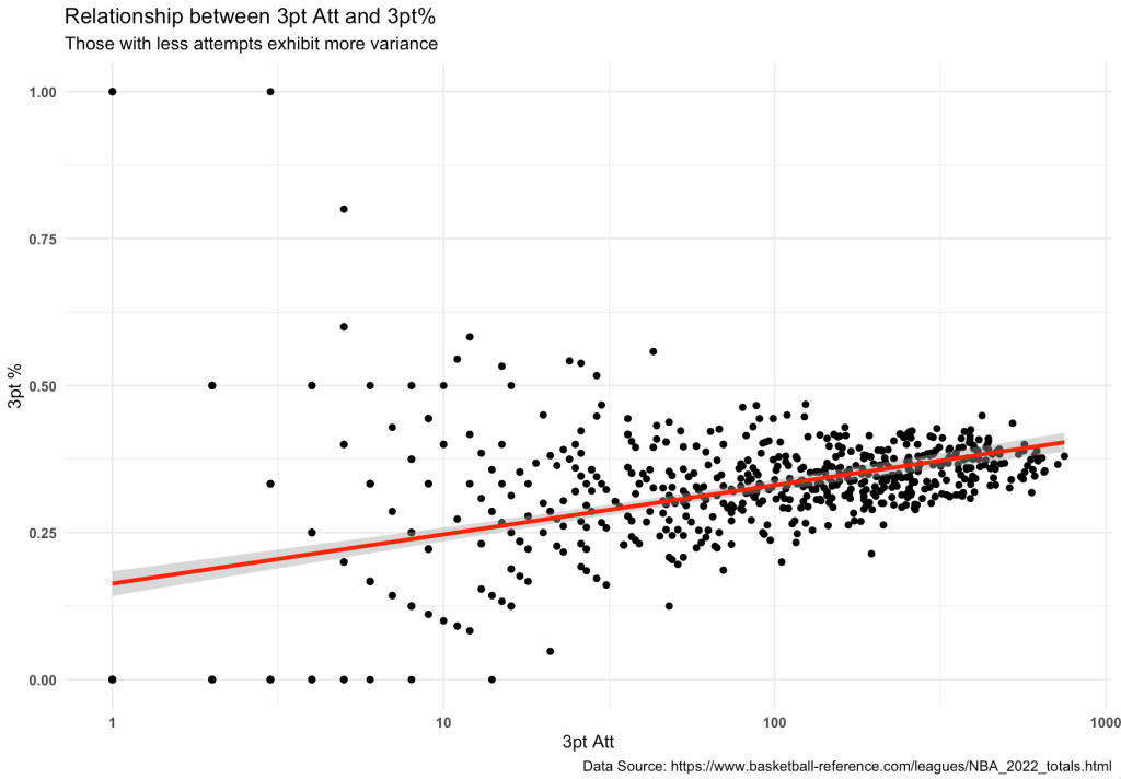
To help wrap our heads around the relationship between 3pt% and 3pt attempts, we will build a simple plot.
Notice that the number of 3 point attempts has some influence on 3pt%. First, as 3pt attempts increase, so does 3pt%. This is because better 3pt shooters will take more 3pt shots and, because they are good, their teams will also try and put them in position to take these shots. Additionally, we can see that as 3pt attempts increase, the amount of variance in performance decreases. Players with under 100 3pt attempts are relatively spread out around the regression line.
Bayesian Shrinkage using the Beta-Binomial Conjugate
As a review from the prior blog article on this topic, we can use our knowledge of the 3pt% success of NBA players as a prior to help shrink observations towards the “expected” outcome. The amount of shrinkage a player exhibits will be dependent on the number of 3pt attempts they have. A smaller sample size means we have less confidence in the observed performance and thus greater shrinkage towards the population prior. Conversely, a large sample size means more confidence in the observed performance and therefore much less shrinkage.
From the prior article we estimated the alpha and beta parameters for our beta distribution to be 61.8 and 106.2, respectively. Recall that these values were estimated from the prior 2 seasons and using only those players with 200 or more 3pt attempts. The alpha and beta parameters provide us with a prior mean for NBA 3pt% of 36.8%.
We will apply this prior knowledge to the observations of all players in our 2022 data set by using the beta-binomial conjugate.
alpha <- 61.8
beta <- 106.2

prior_mu <- alpha / (alpha + beta)
prior_mu

tbl2022 <- tbl2022 %>%
  mutate(three_pt_missed = three_pt_att - three_pt_made,
         posterior_alpha = three_pt_made + alpha,
         posterior_beta = three_pt_missed + beta,
         posterior_three_pt_pct = posterior_alpha / (posterior_alpha + posterior_beta),
         posterior_three_pt_sd = sqrt((posterior_alpha * posterior_beta) / ((posterior_alpha + posterior_beta)^2 * (posterior_alpha + posterior_beta + 1))))
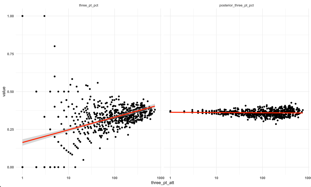
Next, we create a plot to see how the beta-binomial posterior for each player looks relative to the raw data (plotted on the left):
Combining our prior and observed values we can see (on the right) that the data are now constrained around the prior (36.8%). Players with a small number of observations (on the left) are pulled nearest to the line while players with larger observations (on the right) are less influenced by the prior and tend to remain closer to their observed performance.
The problem is that the prior mean (36.8%) is too high for the players with a small number of 3pt attempts. Surely we wouldn’t want to make the assumption that their performance is close to the prior for players that had over 200 attempts! For example, the players with under 50 attempts have an observed average 3pt% of 30% and a median 3pt% of 25% (just over 10% less than those those who had 200 or more attempts!).
To deal with this issue we need to account for shot attempts first so that we can estimate players with smaller sample sizes relative to a prior performance that is more appropriate for them (IE, a prior that is lower than that currently being assumed by our alpha and beta parameters).
Accounting for 3pt Shot Attempts
Our outcome variable is binomial (success and failures) so we will use a beta-binomial regression to estimate a prior for 3pt% while controlling for 3pt shot attempts.
suppressPackageStartupMessages({
  suppressWarnings({
    library(gamlss)
  })
})

fit_3pt <- gamlss(cbind(three_pt_made, three_pt_missed) ~ log(three_pt_att),
                  data = tbl2022,
                  family = BB(mu.link = "identity"))

## extract model coefficients
fit_3pt$mu.coefficients
fit_3pt$sigma.coefficients
Now we can use these model coefficients to fit an estimated 3pt% for each player based on their number of 3pt attempts. This estimation will serve as our prior, which we will then turn into a new posterior 3pt% for each player using our beta-binomial approach. Note that while the mean 3pt% for each player will vary depending on shot attempts the population sigma will be constant for all athletes, representing the variance that we expect all of those in the population to similarly exhibit.
tbl2022 <- tbl2022 %>%
  mutate(mu = fitted(fit_3pt, parameter = "mu"),
         sigma = fitted(fit_3pt, parameter = "sigma"),
         prior_alpha_reg = mu / sigma,
         prior_beta_reg = (1 - mu) / sigma,
         posterior_alpha_reg = prior_alpha_reg + three_pt_made,
         posterior_beta_reg = prior_beta_reg + three_pt_missed,
         posterior_mu_reg = posterior_alpha_reg / (posterior_alpha_reg + posterior_beta_reg))
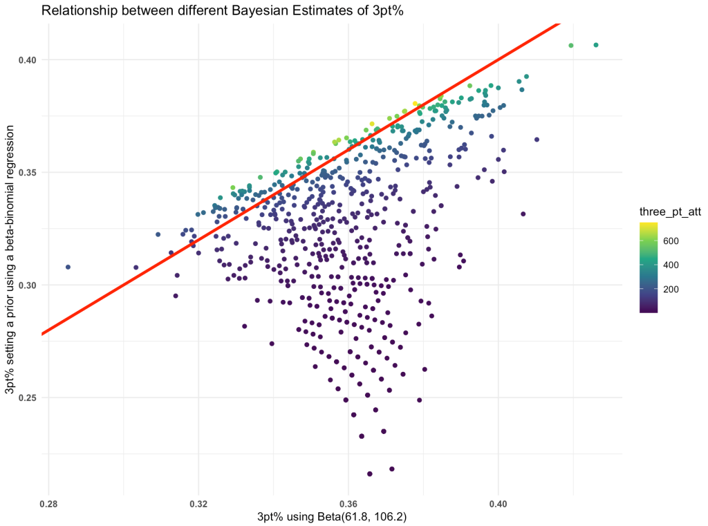
We now have two estimates of each player’s 3pt%. One that was calculated using the beta-binomial conjugate with a prior of 36.8% (the average 3pt% for all shooters with 200 or more 3pt shots). The second estimate first establishes a prior based on the number of 3pt shots the player has taken and then updates that prior based on the individual player’s performance in those shots. We can plot the relationship between these two.

Notice that those with more 3 point attempts are close to the red line (intercept = 0, slope = 1) , representing perfect agreement between the two estimates, while those with less attempts are pulled further down, indicating that we estimate them to be poorer 3pt shooters.
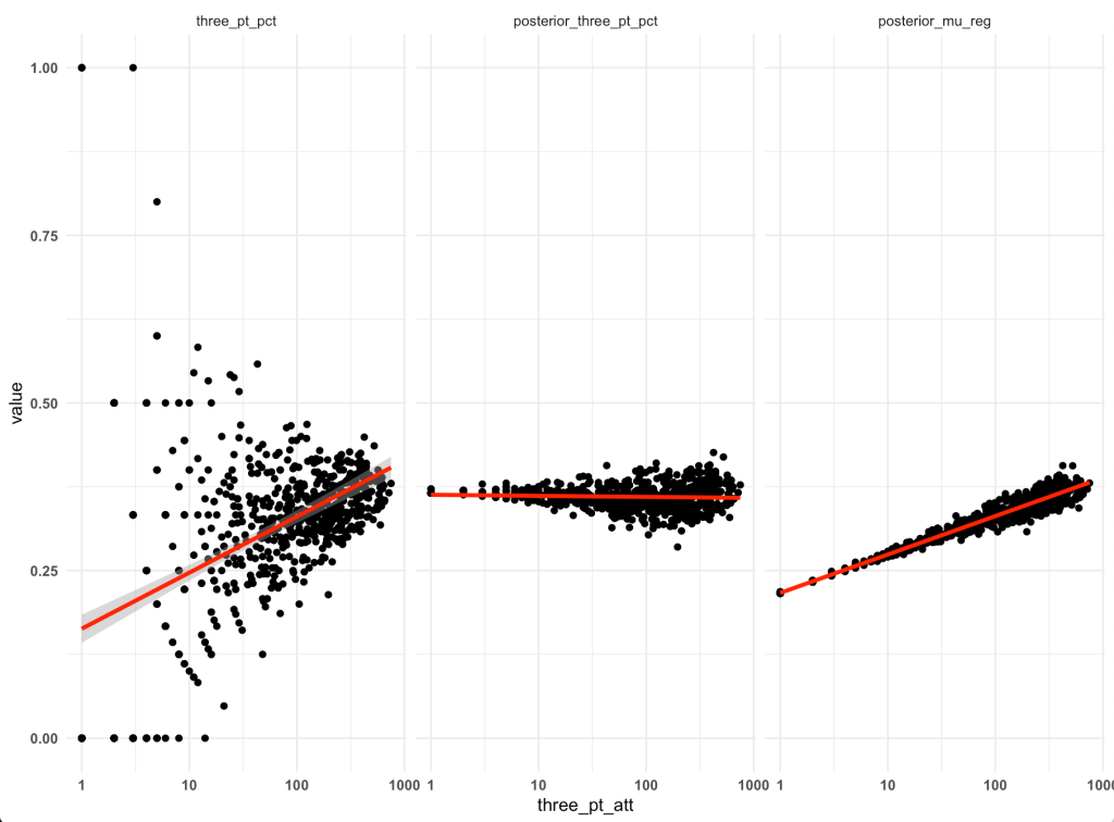
Finally, we can compare the results from our beta-binomial regression prior with our other two estimates of performance (raw observations and our prior of 36.8%).
In the right most plot (beta-binomial regression prior) we see those with a small number of 3pt attempts are shrunk to a smaller prior 3pt% than those with a larger number of 3pt attempts.
Making an estimation for a new player
We can use this approach to estimate the performance of a new player, as well.
new_player <- data.frame( three_pt_att = 10, three_pt_made = 2, three_pt_missed = 10 - 2, three_pt_pct = 2 / 10 ) new_player %>%
  mutate(mu = predict(fit_3pt, newdata = new_player),
         sigma = exp(fit_3pt$sigma.coefficients),
         prior_alpha = mu / sigma,
         prior_beta = (1 - mu) / sigma,
         posterior_alpha = prior_alpha + three_pt_made,
         posterior_beta = prior_beta + three_pt_missed,
         posterior_mu = posterior_alpha / (posterior_alpha + posterior_beta)) %>%
  pivot_longer(cols = everything())
The new player took 10 three point shots, made 2, and has an observed 3pt% of 20%. Using our beta-binomial regression model we estimate the prior for a player with 10 attempts to be 0.274. Combining the prior with the 10 attempts we get a posterior 3pt% for the player of 0.272 (slightly below the average for the population of players who had 10 attempts).
Useful Resources
Some textbooks that I’ve found useful for exploring this type of work:


