As I’ve discussed previously, we sometimes don’t have enough data where doing a train/test split makes sense. As such, we are better off building our model using cross-validation. In previous blog articles, I’ve talked about how to build models using cross-validation within the {tidymodels} framework (see HERE and HERE). In my prior examples, we fit the model over the cross-validation folds and then constructed the final model that we could then use to make predictions with, later on.
Recently, I ran into a situation where I wanted to see what the model coefficients look like across all of the cross-validation folds. So, I decided to make a quick blog post on how to do this, in case it is useful to others.
Load Packages & Data
We will use the {mtcars} package from R and build a regression model, using several independent variables, to predict miles per gallon (mpg).
### Packages -------------------------------------------------------

library(tidyverse)
library(tidymodels)

### Data -------------------------------------------------------

dat <- mtcars dat %>%
  head()
Create Cross-Validation Folds of the Data
I’ll use 10-fold cross validation.
### Modelling -------------------------------------------------------
## Create 10 Cross Validation Folds

set.seed(1)
cv_folds <- vfold_cv(dat, v = 10)
cv_folds
Specify a linear model and set up the model formula
## Specify the linear regression engine
## model specs
lm_spec <- linear_reg() %>%
  set_engine("lm")


## Model formula
mpg_formula <- mpg ~ cyl + disp + wt + drat
Set up the model workflow and fit the model to the cross-validated folds
## Set up workflow
lm_wf <- workflow() %>%
  add_formula(mpg_formula) %>%
  add_model(lm_spec)

## Fit the model to the cross validation folds
lm_fit <- lm_wf %>%
  fit_resamples(
    resamples = cv_folds,
    control = control_resamples(extract = extract_model, save_pred = TRUE)
  )
Extract the model coefficients for each of the 10 folds (this is the fun part!)
Looking at the lm_fit output above, we see that it is a tibble consisting of various nested lists. The id column indicates which cross-validation fold the lists in each row pertain to. The model coefficients for each fold are stored in the .extracts column of lists. Instead of printing out all 10, let’s just have a look at the first 3 folds to see what they look like.
lm_fit$.extracts %>%
  .[1:3]
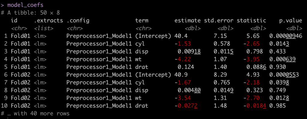
There we see in the .extracts column, <lm> indicating the linear model for each fold. With a series of unnesting we can snag the model coefficients and then put them into a tidy format using the {broom} package. I’ve commented out each line of code below so that you know exactly what is happening.
# Let's unnest this and get the coefficients out
model_coefs <- lm_fit %>%
  select(id, .extracts) %>%                    # get the id and .extracts columns
  unnest(cols = .extracts) %>%                 # unnest .extracts, which produces the model in a list
  mutate(coefs = map(.extracts, tidy)) %>%     # use map() to apply the tidy function and get the coefficients in their own column
  unnest(coefs)                                # unnest the coefs column you just made to get the coefficients for each fold

model_coefs
Now that we have a table of estimates, we can plot the coefficient estimates and their 95% confidence intervals. The term column indicates each variable. We will remove the (Intercept) for plotting purposes.
Plot the Coefficients
## Plot the model coefficients and 2*SE across all folds
model_coefs %>%
  filter(term != "(Intercept)") %>%
  select(id, term, estimate, std.error) %>%
  group_by(term) %>%
  mutate(avg_estimate = mean(estimate)) %>%
  ggplot(aes(x = id, y = estimate)) +
  geom_hline(aes(yintercept = avg_estimate),
             size = 1.2,
             linetype = "dashed") +
  geom_point(size = 4) +
  geom_errorbar(aes(ymin = estimate - 2*std.error, ymax = estimate + 2*std.error),
                width = 0.1,
                size = 1.2) +
  facet_wrap(~term, scales = "free_y") +
  labs(x = "CV Folds",
       y = "Estimate ± 95% CI",
       title = "Regression Coefficients ± 95% CI for 10-fold CV",
       subtitle = "Dashed Line = Average Coefficient Estimate over 10 CV Folds per Independent Variable") +
  theme_classic() +
  theme(strip.background = element_rect(fill = "black"),
        strip.text = element_text(face = "bold", size = 12, color = "white"),
        axis.title = element_text(size = 14, face = "bold"),
        axis.text.x = element_text(angle = 60, hjust = 1, face = "bold", size = 12),
        axis.text.y = element_text(face = "bold", size = 12),
        plot.title = element_text(size = 18),
        plot.subtitle = element_text(size = 16))
Now we can clearly see the model coefficients and confidence intervals for each of the 10 cross validated folds.
Wrapping Up
This was just a quick and easy way of fitting a model using cross-validation to extract out the model coefficients for each fold. Often, this is probably not necessary as you will fit your model, evaluate your model, and be off and running. However, there may be times where more specific interrogation of the model is required or, you might want to dig a little deeper into the various outputs of the cross-validated folds.
All of the code is available on my GitHub page.
If you notice any errors in code, please reach out!


