Simulating data is something I find myself doing all the time. Not only to explore uncertainty in data but also to explore model assumptions, understand how models behave under different circumstances, or to try and understand how a future analysis might work given some underlying data generating process. Thus, I decided to put together a series on simulations and resampling using R (I’ll also add a few analog scripts using Python to the GitHub repository).
In Part 1, I’ll provide some thoughts around why you might want to simulate or resample data and then show how you can simply do this in R. Additionally, I’ll walk through several helper functions for conducting and summarizing simulations/resamples as well as some basics around for() and while() loops, as we will use these extensively in our simulation and resampling processes.
My Github repository will contain all of the scripts in this series.
Why do we simulate or resample data?
- The data generating process is what defines the properties of our data and dictates the type of distribution we are dealing with. For example, the mean and standard deviation reflect the two parameters of the data generating process for a normal distribution. We rarely know what the data generating process of our data is in the real world, thus we must infer it from our sample data. Both resampling and simulation offer methods of understanding the data generating process of data.
- Sample data represents a small sliver of what might be occurring in the broader population. Using resampling and simulation, we are able to build larger data sets based on information contained in the sample data. Such approaches allow us to explore our uncertainty around what we have observed in our sample and the inferences we might be able to make about that larger population.
- Creating samples of data allows us to assess patterns in the data and evaluate those patterns under different circumstances, which we can directly program.
- By coding a simulation, we are able to reflect a desired data generating process, allowing us to evaluate assumptions or limitations of data that we have collected or are going to collect.
- The world is full of randomness, meaning that every observation we make comes with some level of uncertainty. The uncertainty that we have about the true value of our observation can be expressed via various probability distributions. Resamping and simulation are ways that we can mimic this randomness in the world and help calibrate our expectation about the probability of certain events or observations occurring.
Difference between resampling and simulation
Resampling and simulation are both useful at generating data sets and reflecting uncertainty. However, they accomplish this task in different ways.
- Resampling deals with techniques that take the observed sample data and randomly draw observations from that data to construct a new data set. This is often done thousands of times, building thousands of new data sets, and then summary statistics are produced on those data sets as a means of understanding the data generating properties.
- Simulation works by assuming a data generating process (e.g., making a best guess or estimating a plausible mean and standard deviation for the population from previous literature) and then generating multiple samples of data, randomly, from the data generating process features.
Sampling from common distributions
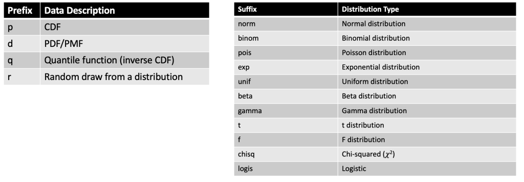
To create a distribution in R we can use any one of the four primary prefixes, which define the type of information we want returned about the distribution, followed by the suffix that defines the distribution we are interested in.
Here is a helpful cheat sheet I put together for some of the common distributions one might use:
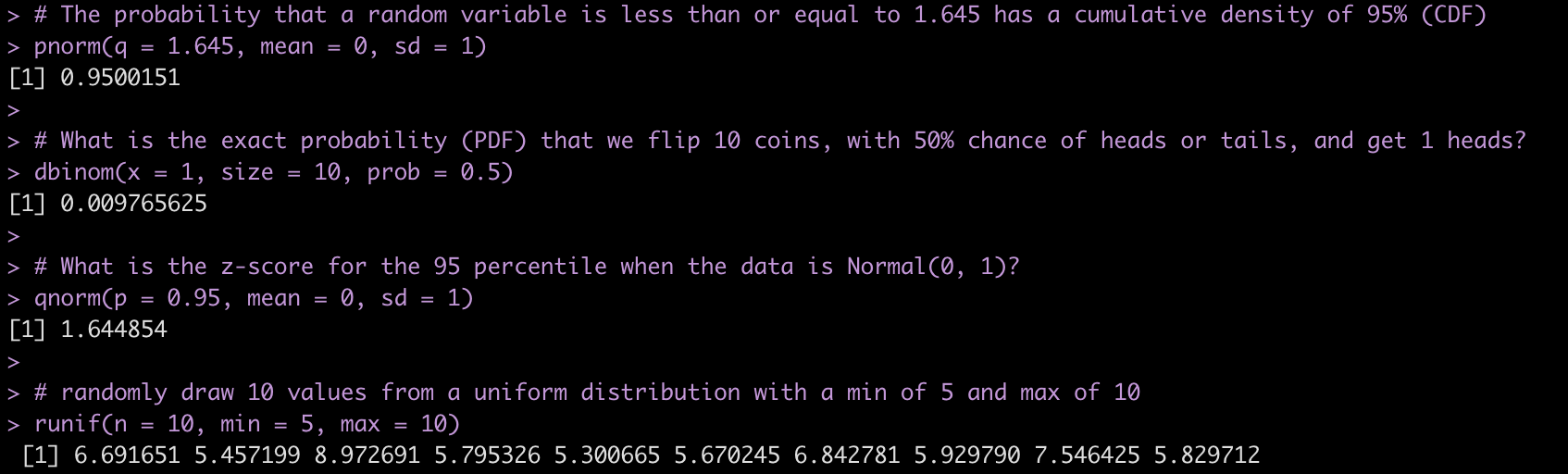
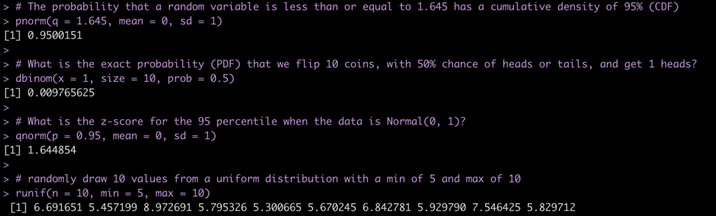
Some examples:
# The probability that a random variable is less than or equal to 1.645 has a cumulative density of 95% (CDF)
pnorm(q = 1.645, mean = 0, sd = 1)

# What is the exact probability (PDF) that we flip 10 coins, with 50% chance of heads or tails, and get 1 heads?
dbinom(x = 1, size = 10, prob = 0.5)

# What is the z-score for the 95 percentile when the data is Normal(0, 1)?
qnorm(p = 0.95, mean = 0, sd = 1)

# randomly draw 10 values from a uniform distribution with a min of 5 and max of 10
runif(n = 10, min = 5, max = 10)
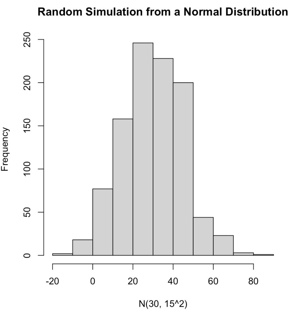
We can completely simulate different distributions and properties of those distributions using these function. For several examples of different distributions see the GitHub code. Below is an example of 1,000 random observations from a normal distribution with a mean of 30 and standard deviation of 15 and plot the results..
## set the seed for reproducibility
set.seed(10)
norm_dat <- rnorm(n = 1000, mean = 30, sd = 15)

hist(norm_dat,
     main = "Random Simulation from a Normal Distribution",
     xlab = "N(30, 15^2)")
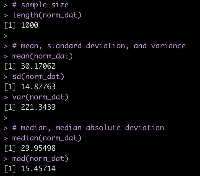
We can produce a number of summary statistics on this vector of random values:
# sample size
length(norm_dat)

# mean, standard deviation, and variance
mean(norm_dat)
sd(norm_dat)
var(norm_dat)

# median, median absolute deviation
median(norm_dat)
mad(norm_dat)
for & while loops
Typically, we are going to want to resample data more than once or to run multiple simulations. Often, we will want to do this thousands of times. We can use R to help us in the endeavor by programming for() and while() loops to do the heavy lifting for us and store the results in a convenient format (e.g., vector, data frame, matrix, or list) so that we can summarize it later.
for loops
for() loops are easy ways to tell `R` that we want it to do some sort of task for a specified number of iterations.
For example, let’s create a for() loop that adds 5 for every value from 1 to 10, for(i in 1:10).
# program the loop to add 5 to every value from 1:10
for(i in 1:10){

  print(i + 5)

}
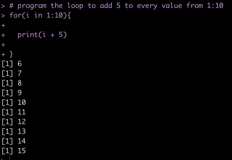
We notice that the result is printed directly to the console. If we are doing thousands of iterations or if we want to store the results to plot and summarize them later, this wont be a good option. Instead, we can allocate an empty vector or data frame to store these values.
## storing values as vector
n <- 10
vector_storage <- rep(NA, times = n)
for(i in 1:n){
vector_storage[i] <- i + 5
}
vector_storage
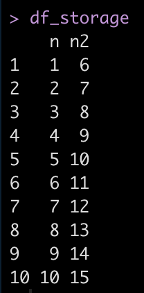
## store results back to a data frame
n <- 10
df_storage <- data.frame(n = 1:10)
for(i in 1:n){
df_storage$n2[i] <- i + 5
}
df_storage
while loops
while() loops differ from for() loops in that they continue to perform a process while some condition is met.
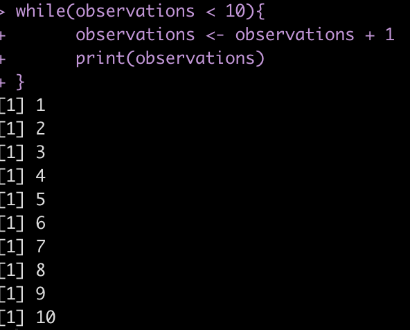
For example, if we start with a count of 0 observations and continually add 1 observation we want to perform this process as long as the observations are below 10.
observations <- 0

while(observations < 10){
	observations <- observations + 1
	print(observations)
}
We can also use while() loops to test logical arguments.
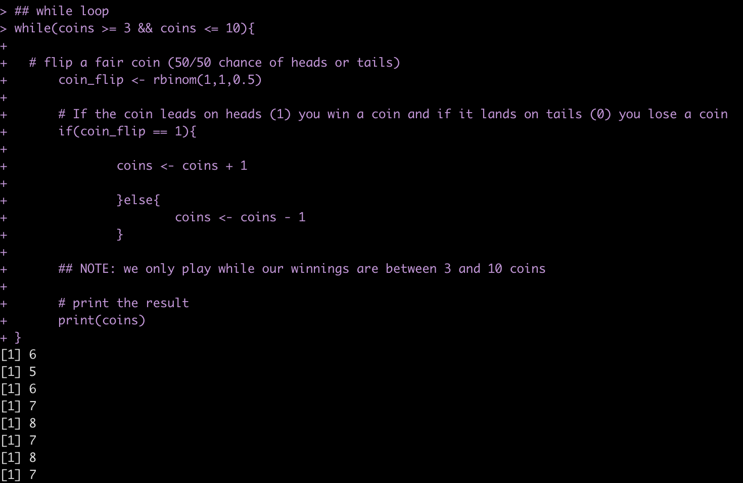
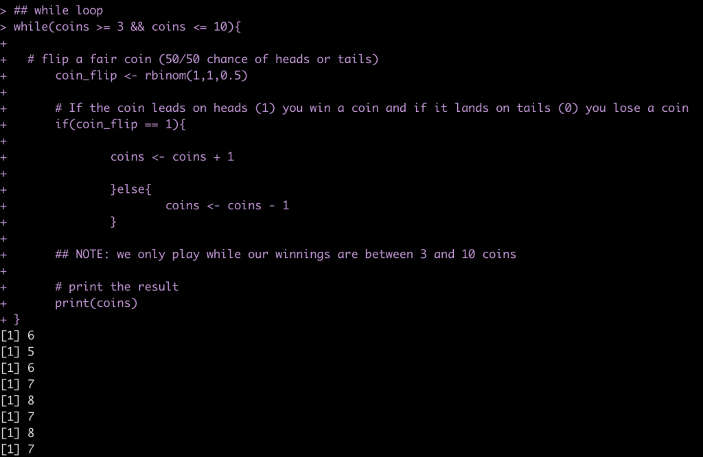
For example, let’s say we have five coins in our pocket and want to play a game with a fried where we flip a fair coin and every time it ends on heads (coin_flip == 1) we get a coin and every time it ends on tails we lose a coin. We are only willing to continue playing the game as long as retain between 3 and 10 coins.
## starting number of coins
coins <- 5

## while loop
while(coins >= 3 && coins <= 10){

  # flip a fair coin (50/50 chance of heads or tails)
	coin_flip <- rbinom(1,1,0.5)

	# If the coin leads on heads (1) you win a coin and if it lands on tails (0) you lose a coin
	if(coin_flip == 1){

		coins <- coins + 1

		}else{
			coins <- coins - 1
		}

	## NOTE: we only play while our winnings are between 3 and 10 coins

	# print the result
	print(coins)
}
You can run the code many times and find out, on average, how many flips you will get!
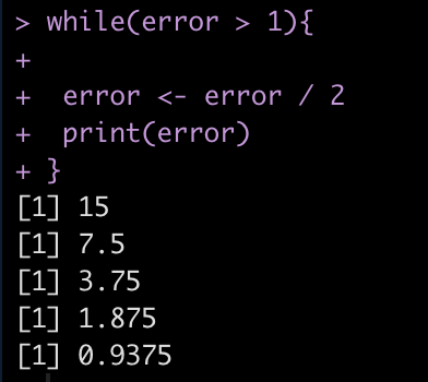
Finally, we can also use while() loops if we are building models to minimize error. For example, lets say we have an error = 30 and we want to continue running the code until we have minimized the error below 1. So, the code will run while(error > 1).
error <- 30 while(error > 1){

 error <- error / 2
 print(error)
}
Helper functions for summarizing distributions
There are a number of helper functions in base R that can assist us in summarizing data.
- apply() will return your results in a vector
- lapply() will return your results as a list
- sapply() can return the results as a vector or a list (if you set the argument `simplify = FALSE`)
- tapply() will return your results in a named vector based on whichever grouping variable you specify
## create fake data
set.seed(1234)
fake_dat <- data.frame(
group = rep(c("a", "b", "c"), each = 5),
x = rnorm(n = 15, mean = 10, sd = 2),
y = rnorm(n = 15, mean = 30, sd = 10),
z = rnorm(n = 15, mean = 75, sd = 20)
)
fake_dat
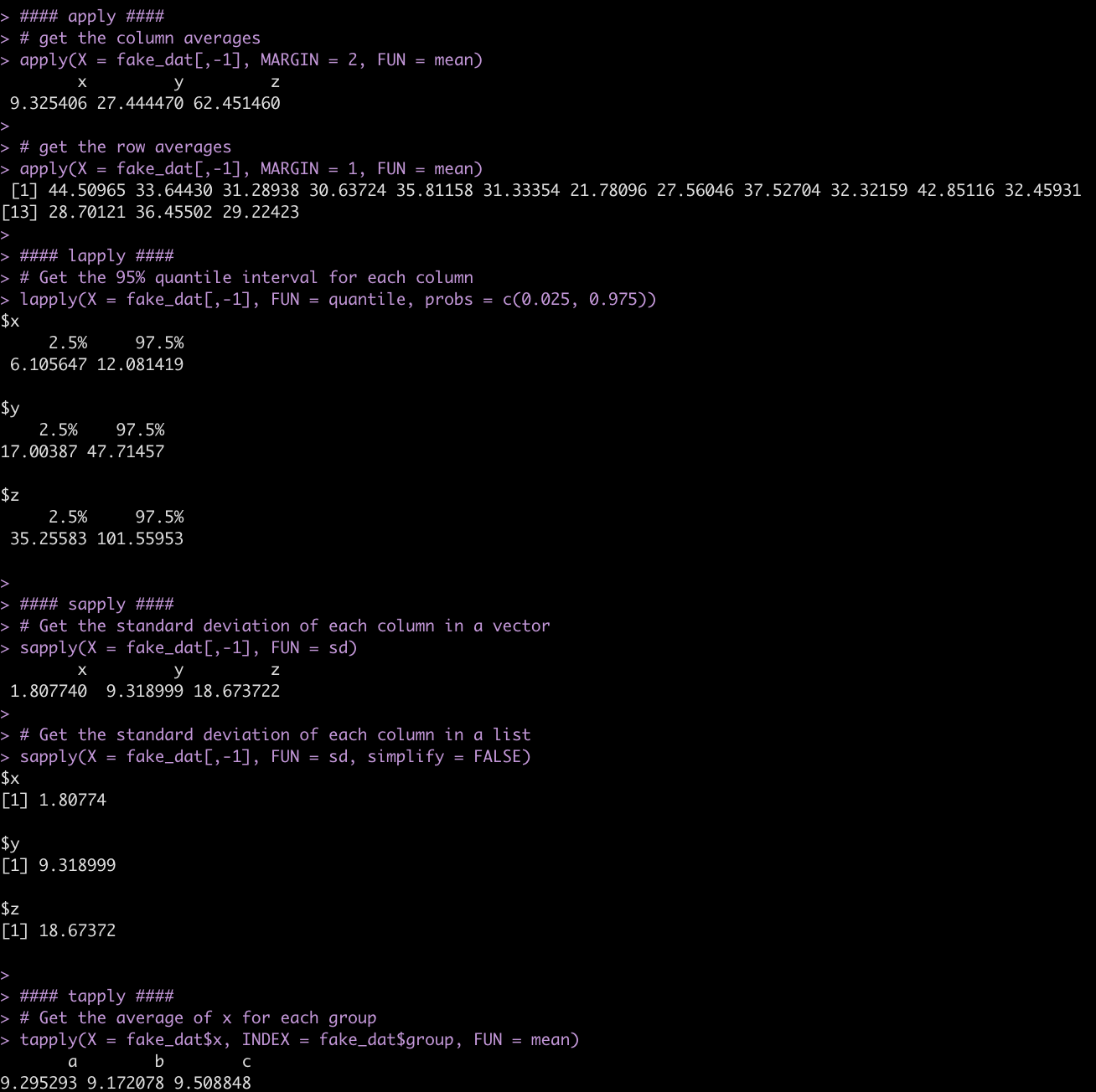
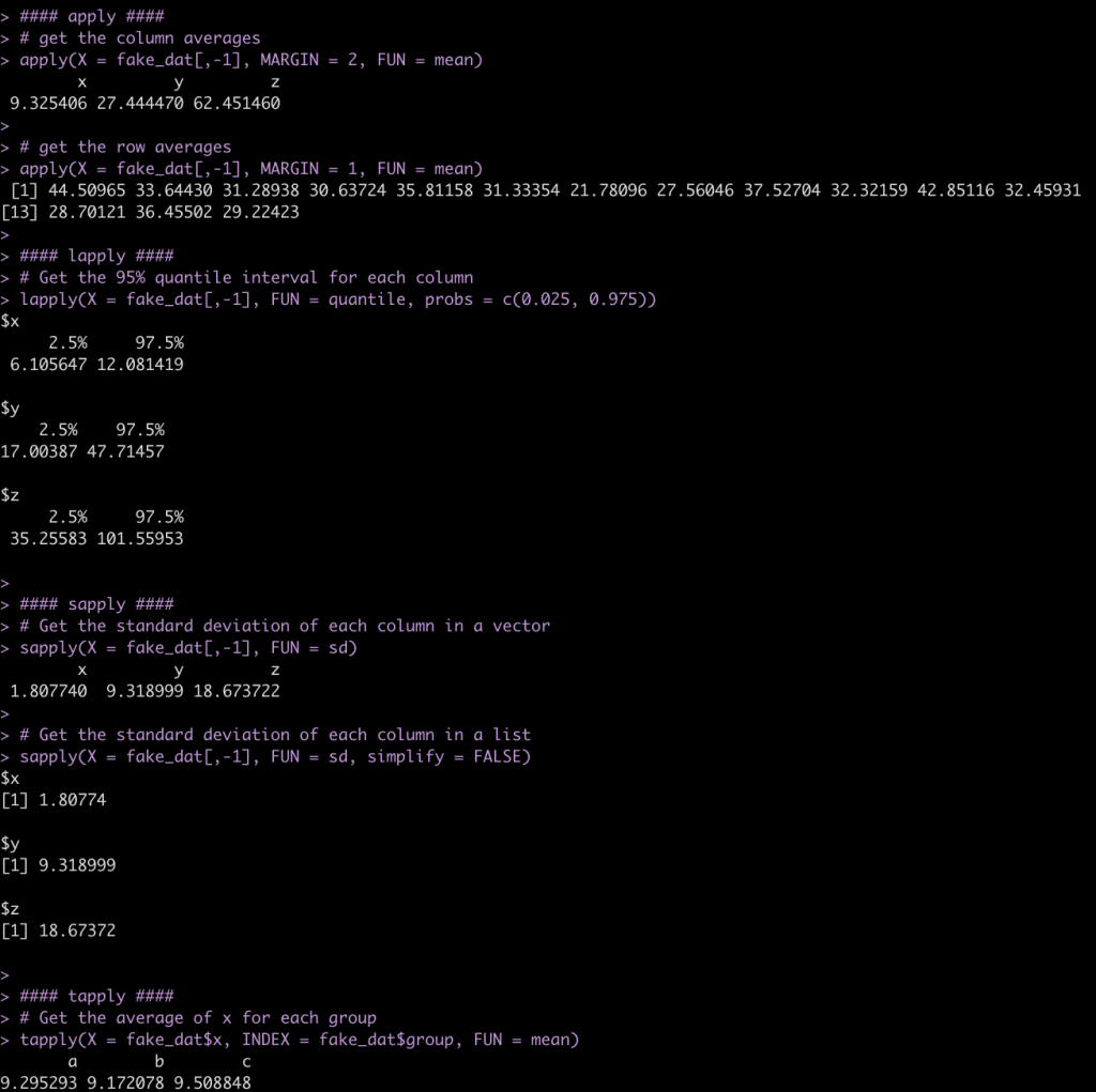
#### apply ####
# get the column averages
apply(X = fake_dat[,-1], MARGIN = 2, FUN = mean)
# get the row averages
apply(X = fake_dat[,-1], MARGIN = 1, FUN = mean)
#### lapply ####
# Get the 95% quantile interval for each column
lapply(X = fake_dat[,-1], FUN = quantile, probs = c(0.025, 0.975))
#### sapply ####
# Get the standard deviation of each column in a vector
sapply(X = fake_dat[,-1], FUN = sd)
# Get the standard deviation of each column in a list
sapply(X = fake_dat[,-1], FUN = sd, simplify = FALSE)
#### tapply ####
# Get the average of x for each group
tapply(X = fake_dat$x, INDEX = fake_dat$group, FUN = mean)
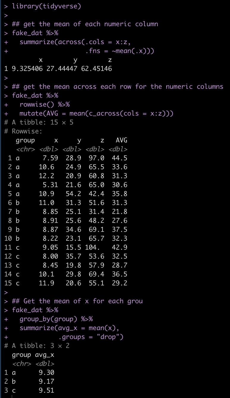
We can alternatively do a lot of this type of data summarizing using the convenient R package {tidyverse}.
library(tidyverse)

## get the mean of each numeric column
fake_dat %>%
  summarize(across(.cols = x:z,
                   .fns = ~mean(.x)))

## get the mean across each row for the numeric columns
fake_dat %>%
  rowwise() %>%
  mutate(AVG = mean(c_across(cols = x:z)))

## Get the mean of x for each grou
fake_dat %>%
  group_by(group) %>%
  summarize(avg_x = mean(x),
            .groups = "drop")

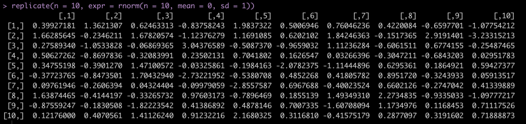
Finally, another handy base R function is replicate(), which allows us to replicate a task n number of times.
For example, let’s say we want to draw from a random normal distribution, rnorm() with a mean = 0 and sd = 1 but, we want to run this random simulation 10 times and get 10 different data sets. replicate()` allows us to do this and stores the results in a matrix with 10 columns, each with 10 rows of the random sample.
replicate(n = 10, expr = rnorm(n = 10, mean = 0, sd = 1))
Wrapping Up
In this first part of my simulation and resampling series we went through some of the key functions in R that will help us build the scaffolding for our future work. In Part 2, we we dive into bootstrap resampling and simulating bivariate and multivariate normal distributions.
All code is available in both rmarkdown and html format on my Github page.