We’ve built up a number of simulations over the 7 articles in this series. The last few articles have been looking at linear regression and simulating different intricacies in the data that allow us to explore model assumptions. To end this series, we will now extend the linear model to a mixed model. We will start by building a linear regression model and go through the steps of simulation to build up the hierarchical structure of the data.

For those interesting here are the previous 7 articles in this series:

• Part 1 discussed the basic functions for simulating and sampling data in R
• Part 2 walked us through how to perform bootstrap resampling and then simulate bivariate and multivariate distributions
• Part 3 we worked making group comparisons by simulating thousands of t-tests
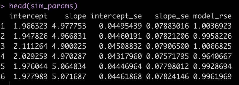
• Part 4 building simulations for linear regression
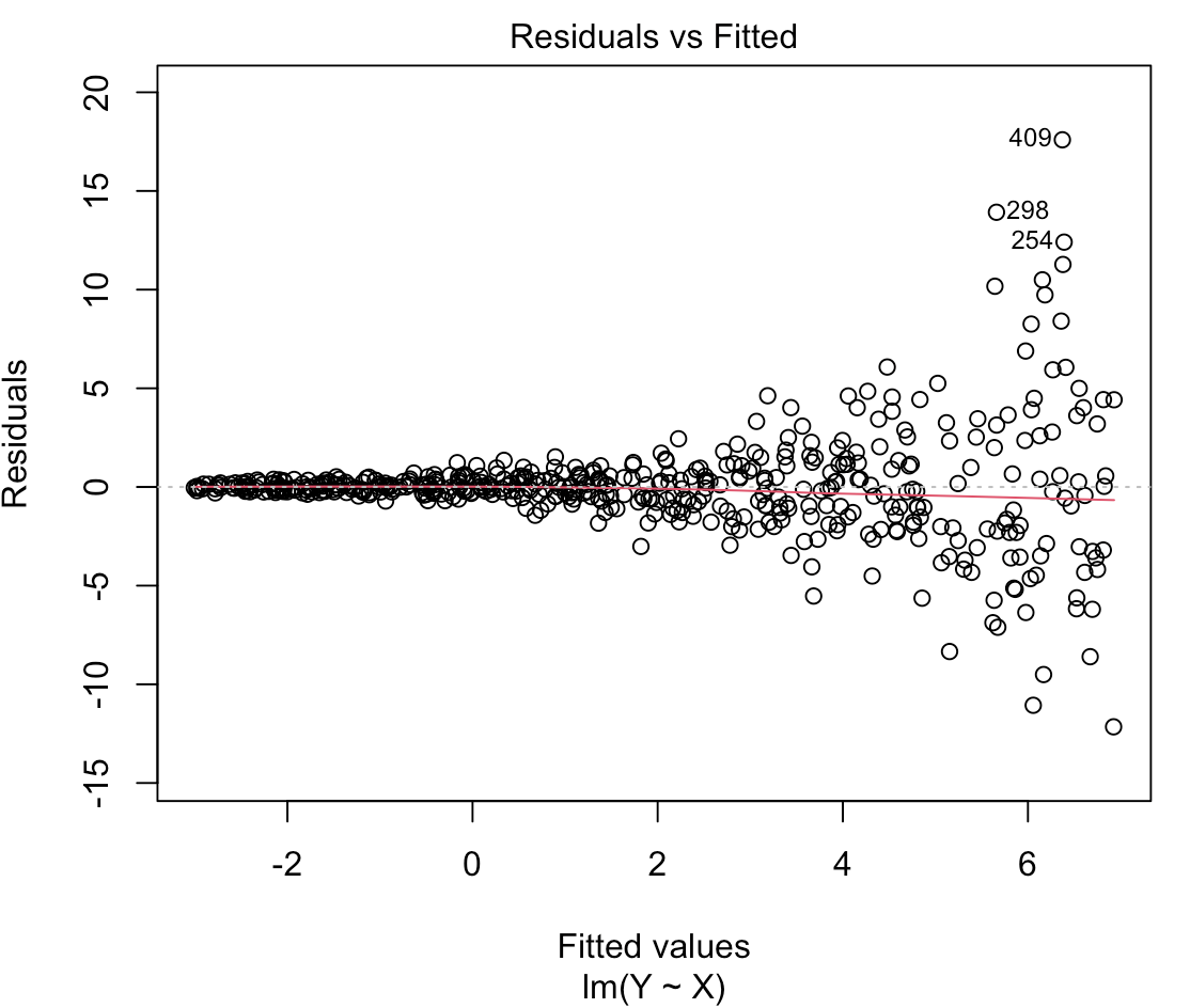
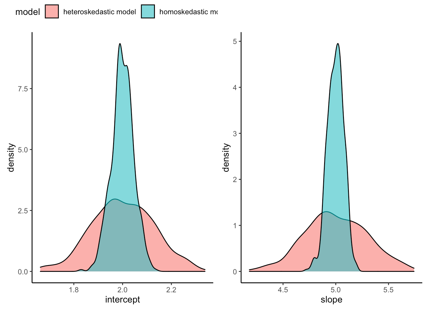
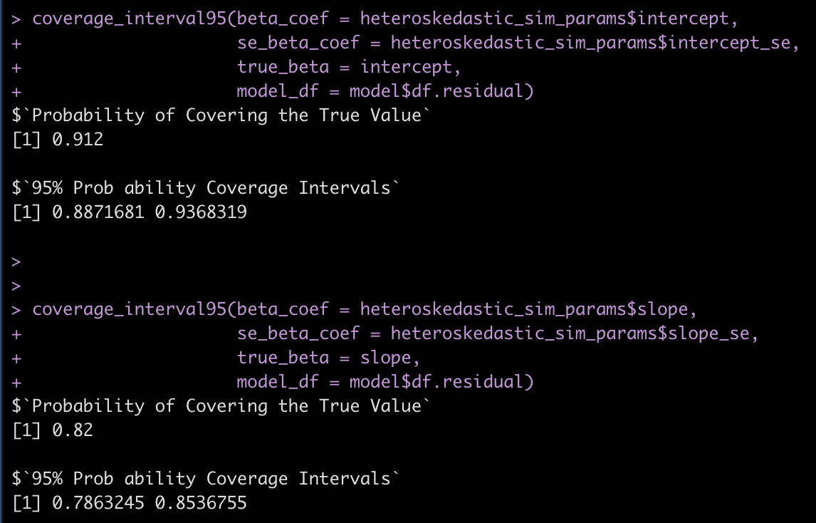
• Part 5 using simulation to investigate the homoskedasticity assumption in regression
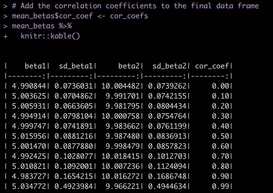
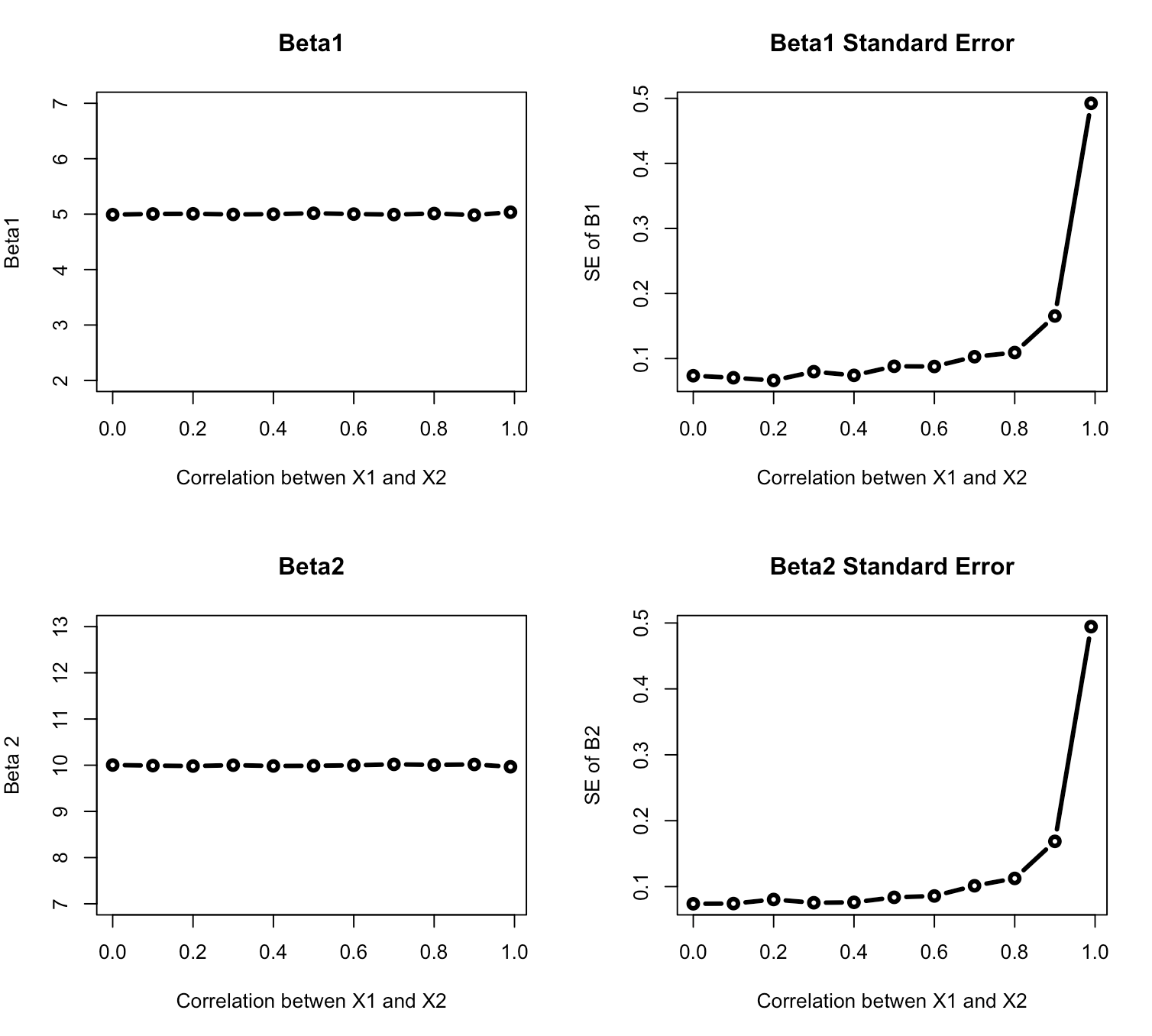
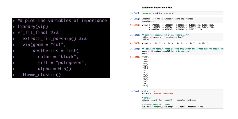
• Part 6 using simulation to investigate the multicollinearity assumption in regression
• Part 7 simulating measurement error in regression

As always, complete code for this article is available on my GitHub page.

Side Note: This is a very code heavy article as the goal is to show not only simulations of data and models but how to extract the model parameters from the list of simulations. As such, this a rather long article with minimal interpretation of the models.

First a linear model

Our data will look at training load for 10 players in two different positions, Forwards (F) and Mids (M). The Forwards will be simulated to have less training load than the Mids and we will add some random error around the difference in these group means. We will simulate this as a linaer model where b0 represents the model intercept and is the mean value for Forwards and b1 represents the coefficient for when the group is Mids.

library(tidyverse)
library(broom)
library(lme4)

theme_set(theme_light())
## Model Parameters
n_positions <- 2
n_players <- 10
b0 <- 80
b1 <- 20
sigma <- 10

## Simulate
set.seed(300)
pos <- rep(c("M", "F"), each = n_players)
player_id <- rep(1:10, times = 2)
model_error <- rnorm(n = n_positions*n_players, mean = 0, sd = sigma)
training_load <- b0 + b1 * (pos == "M") + model_error

d <- data.frame(pos, player_id, training_load)
d

Calculate some summary statistics

d %>%
  ggplot(aes(x = pos, y = training_load)) +
  geom_boxplot()

d %>%
  group_by(pos) %>%
  summarize(N = n(),
            avg = mean(training_load),
            sd = sd(training_load)) %>%
  mutate(se = sd / sqrt(N)) %>%
  knitr::kable()

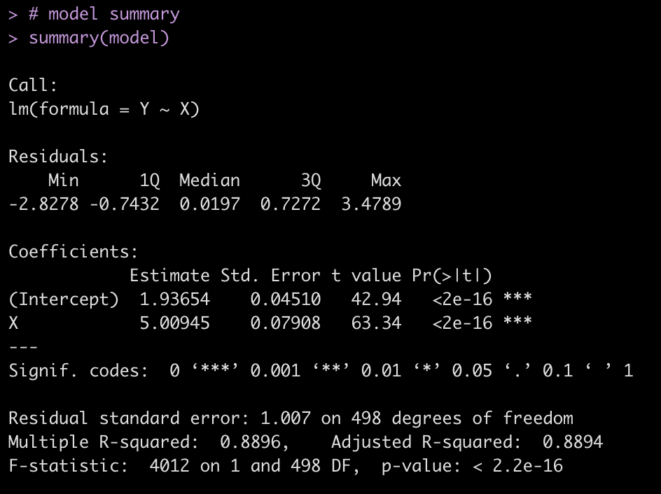
Build a linear model

fit <- lm(training_load ~ pos, data = d)
summary(fit)

Now, we wrap all the steps in a function so that we can use replicate() to create thousands of simulations or to change parameters of our simulation. The end result of the function is going to be the linear regression model.

sim_func <- function(n_positions = 2, n_players = 10, b0 = 80, b1 = 20, sigma = 10){

  ## simulate data
  pos <- rep(c("M", "F"), each = n_players)
  player_id <- rep(1:10, times = 2)
  model_error <- rnorm(n = n_positions*n_players, mean = 0, sd = sigma)
  training_load <- b0 + b1 * (pos == "M") + model_error

  ## store in data frame
  d <- data.frame(pos, player_id, training_load)
  
  ## construct linear model
  fit <- lm(training_load ~ pos, data = d)
  summary(fit)
}

Try the function out with the default parameters

sim_func()

Use replicate() to create many simulations.

Doing this simulation once doesn’t help us. We want to be able to do this thousands of times. All of the articles in this series have used for() loops up until this point. But, if you recall the first article in the series where I laid out several helpful functions for coding simulations, I showed an example of the replicate() function, which will take a function and run it’s result for as many times as you specify. I found this function while I was working through the simulation chapter of Gelman et al’s book, Regression and Other Stories. I think in cases like a mixed model simulation, where you can have many layers and complexities to the data, writing a simple function and then replicating it thousands of times is much easier to debug and much cleaner for others to read than having a bunch of nested for() loops.

Technical Note: We specify the argument simplify = FALSE so that the results are returned in a list format. This makes more sense since the results are the regression summary results and not a data frame.

team_training <- replicate(n = 1000,
                  sim_func(),
                  simplify = FALSE)

Coefficient Results

team_training %>%
  map_df(tidy) %>%
  select(term, estimate) %>%
  ggplot(aes(x = estimate, fill = term)) +
  geom_density() +
  facet_wrap(~term, scales = "free_x")

team_training %>%
  map_df(tidy) %>%
  select(term, estimate) %>%
  group_by(term) %>%
  summarize(avg = mean(estimate),
            SD = sd(estimate))

Compare the simulated results to the results of the original model fit.

tidy(fit)

Model fit parameters

team_training %>%
  map_df(glance) %>%
  select(adj.r.squared, sigma) %>%
  summarize(across(.cols = everything(),
                   ~mean(.x)))

Compare these results to the original fit

fit %>% 
  glance()

Mixed Model 1

Now that we have the general frame work for building a simulation function and using replicate() we will to build a mixed model simulation.

Above we had a team with two positions groups and individual players nested within those position groups. In this mixed model, we will add a second team so that we can explore hierarchical data.

We will simulate data from 3 teams, each with 2 positions (Forward & Mid). This is a pretty simple mixed model. We will build a more complex one after we get a handle on the code below.

## Model Parameters
n_teams <- 3
n_positions <- 2
n_players <- 10

team1_fwd_avg <- 130
team1_fwd_sd <- 15
team1_mid_avg <- 100
team1_mid_sd <- 5

team2_fwd_avg <- 150
team2_fwd_sd <- 20
team2_mid_avg <- 90
team2_mid_sd <- 10

team3_fwd_avg <- 180
team3_fwd_sd <- 15
team3_mid_avg <- 150
team3_mid_sd <- 15


## Simulated data frame
team <- rep(c("Team1","Team2", "Team3"), each = n_players * n_positions)
pos <- c(rep(c("M", "F"), each = n_players), rep(c("M", "F"), each = n_players), rep(c("M", "F"), each = n_players))
player_id <- as.factor(round(seq(from = 100, to = 300, length = length(team)), 0))

d <- data.frame(team, pos, player_id) d %>%
  head()

# simulate training loads
set.seed(555)
training_load <- c(rnorm(n = n_players, mean = team1_mid_avg, sd = team1_mid_sd), rnorm(n = n_players, mean = team1_fwd_avg, sd = team1_fwd_sd), rnorm(n = n_players, mean = team2_mid_avg, sd = team2_mid_sd), rnorm(n = n_players, mean = team2_fwd_avg, sd = team2_fwd_sd), rnorm(n = n_players, mean = team3_mid_avg, sd = team3_mid_sd), rnorm(n = n_players, mean = team3_fwd_avg, sd = team3_fwd_sd)) d ,- d %>%
  bind_cols(training_load = training_load) 

d %>%
  head()

Calculate summary statistics

## Average training load by team
d %>%
  group_by(team) %>%
  summarize(avg = mean(training_load),
            SD = sd(training_load))

## Average training load by pos
d %>%
  group_by(pos) %>%
  summarize(avg = mean(training_load),
            SD = sd(training_load))

## Average training load by team & position
d %>%
  group_by(team, pos) %>%
  summarize(avg = mean(training_load),
            SD = sd(training_load)) %>%
  arrange(pos)

## Plot
d %>%
  ggplot(aes(x = training_load, fill = team)) +
  geom_density(alpha = 0.5) +
  facet_wrap(~pos)

Construct the mixed model and evaluate the outputs

## Mixed Model
fit_lmer <- lmer(training_load ~ pos + (1 |team), data = d)
summary(fit_lmer)
coef(fit_lmer)
fixef(fit_lmer)
ranef(fit_lmer)
sigma(fit_lmer)
hist(residuals(fit_lmer))

Write a mixed model function

sim_func_lmer <- function(n_teams = 3, 
                          n_positions = 2, 
                          n_players = 10, 
                          team1_fwd_avg = 130,
                          team1_fwd_sd = 15,
                          team1_mid_avg = 100,
                          team1_mid_sd = 5,
                          team2_fwd_avg = 150,
                          team2_fwd_sd = 20,
                          team2_mid_avg = 90,
                          team2_mid_sd = 10,
                          team3_fwd_avg = 180,
                          team3_fwd_sd = 15,
                          team3_mid_avg = 150,
                          team3_mid_sd = 15){

        ## Simulated data frame
        team <- rep(c("Team1","Team2", "Team3"), each = n_players * n_positions)
        pos <- c(rep(c("M", "F"), each = n_players), rep(c("M", "F"), each = n_players), rep(c("M", "F"), each = n_players))
        player_id <- as.factor(round(seq(from = 100, to = 300, length = length(team)), 0))
        
        d <- data.frame(team, pos, player_id)

        # simulate training loads
        training_load <- c(rnorm(n = n_players, mean = team1_mid_avg, sd = team1_mid_sd),
                   rnorm(n = n_players, mean = team1_fwd_avg, sd = team1_fwd_sd),
                   rnorm(n = n_players, mean = team2_mid_avg, sd = team2_mid_sd),
                   rnorm(n = n_players, mean = team2_fwd_avg, sd = team2_fwd_sd),
                   rnorm(n = n_players, mean = team3_mid_avg, sd = team3_mid_sd),
                   rnorm(n = n_players, mean = team3_fwd_avg, sd = team3_fwd_sd))
  
        ## construct the mixed model
  fit_lmer <- lmer(training_load ~ pos + (1 |team), data = d)
  summary(fit_lmer)
}

Try out the function

sim_func_lmer()

Now use replicate() and create 1000 simulations of the model and look at the first model in the list

team_training_lmer <- replicate(n = 1000,
                  sim_func_lmer(),
                  simplify = FALSE)

## look at the first model in the list
team_training_lmer[[1]]$coefficient

Store the coefficient results of the 1000 simulations in a data frame, create plots of the model coefficients, and compare the results of the simulation to the original mixed model.

lmer_coef <- matrix(NA, ncol = 5, nrow = length(team_training_lmer))
colnames(lmer_coef) <- c("intercept", "intercept_se", "posM", "posM_se", 'model_sigma')

for(i in 1:length(team_training_lmer)){
  
  lmer_coef[i, 1] <- team_training_lmer[[i]]$coefficients[1]
  lmer_coef[i, 2] <- team_training_lmer[[i]]$coefficients[3]
  lmer_coef[i, 3] <- team_training_lmer[[i]]$coefficients[2]
  lmer_coef[i, 4] <- team_training_lmer[[i]]$coefficients[4]
  lmer_coef[i, 5] <- team_training_lmer[[i]]$sigma
  
}

lmer_coef <- as.data.frame(lmer_coef) head(lmer_coef) ## Plot the coefficient for position lmer_coef %>%
  ggplot(aes(x = posM)) +
  geom_density(fill = "palegreen")

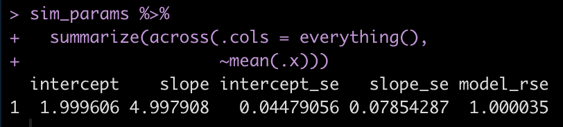
## Summarize the coefficients and their standard errors for the simulations
lmer_coef %>% 
  summarize(across(.cols = everything(),
                   ~mean(.x)))

## compare to the original model
broom.mixed::tidy(fit_lmer)
sigma(fit_lmer)

Extract the random effects for the intercept and the residual for each of the simulated models

ranef_sim <- matrix(NA, ncol = 2, nrow = length(team_training_lmer))
colnames(ranef_sim) <- c("intercept_sd", "residual_sd")

for(i in 1:length(team_training_lmer)){
  
  ranef_sim[i, 1] <- team_training_lmer[[i]]$varcor %>% as.data.frame() %>% select(sdcor) %>% slice(1) %>% pull(sdcor)
  ranef_sim[i, 2] <- team_training_lmer[[i]]$varcor %>% as.data.frame() %>% select(sdcor) %>% slice(2) %>% pull(sdcor)
  
}

ranef_sim <- as.data.frame(ranef_sim) head(ranef_sim) ## Summarize the results ranef_sim %>%
  summarize(across(.cols = everything(),
                   ~mean(.x)))

## Compare with the original model
VarCorr(fit_lmer)

Mixed Model 2

Above was a pretty simple model, just to get our feet wet. Let’s create a more complicated model. Usually in sport and exercise science we have repeated measures of individuals. Often, researchers will set the individual players as random effects with the fixed effects being the component that the researcher is attempting to make an inference about.

In this example, we will set up a team of 12 players with three positions (4 players per position): Forward, Mid, Defender. The aim is to explore the training load differences between position groups while accounting for repeated observations of individuals (in this case, each player will have 20 training sessions). Similar to our first regression model, we will build a data frame of everything we need and then calculate the outcome variable (training load) with a regression model using parameters that we specify. To make this work, we will need to specific an intercept and slope for the position group and an intercept and slope for the individual players as well as a model sigma value. Once we’ve done that, we will fit a mixed model, write a function, and then create 1000 simulations.

## Set up the data frame
n_pos <- 3
n_players <- 12
n_obs <- 20
players <- as.factor(round(seq(from = 100, to = 300, length = n_players), 0))


dat <- data.frame( player_id = rep(players, each = n_obs), pos = rep(c("Fwd", "Mid", "Def"), each = n_players/n_pos * n_obs), training_day = rep(1:n_obs, times = n_players) ) dat %>%
  head()

## Create model parameters
# NOTE: Defender will be the intercept
set.seed(6687)
pos_intercept <- 150
posF_coef <- 170
posM_coef <- -70
individual_intercept <- 50
individual_slope <- 10
sigma <- 10
model_error <- rnorm(n = nrow(dat), mean = 0, sd = sigma)


## we will also create some individual player variance
individual_player_variance <- c()

for(i in players){

  individual_player_variance[i] <- rnorm(n = 1, 
                  mean = runif(min = 2, max = 10, n = 1), 
                  sd = runif(min = 2, max = 5, n = 1))
  
}

individual_player_variance <- rep(individual_player_variance, each = n_obs)

dat$training_load <- pos_intercept + posF_coef * (dat$pos == "Fwd") + posM_coef * (dat$pos == "Mid") + individual_intercept + individual_slope * individual_player_variance + model_error dat %>%
  head()

Calculate summary stats

## Average training load by pos
dat %>%
  group_by(pos) %>%
  summarize(avg = mean(training_load),
            SD = sd(training_load))

## Plot
dat %>%
  ggplot(aes(x = training_load, fill = pos)) +
  geom_density(alpha = 0.5)

Construct the mixed model and evaluate the output

## Mixed Model
fit_lmer_pos <- lmer(training_load ~ pos + (1 | player_id), data = dat)
summary(fit_lmer_pos)
coef(fit_lmer_pos)
fixef(fit_lmer_pos)
ranef(fit_lmer_pos)
sigma(fit_lmer_pos)
hist(residuals(fit_lmer_pos))

Create a function for the simulation

sim_func_lmer2 <- function(n_pos = 3,
                          n_players = 12,
                          n_obs = 20,
                          pos_intercept = 150,
                          posF_coef = 170,
                          posM_coef = -70,
                          individual_intercept = 50,
                          individual_slope = 10,
                          sigma = 10){
  
  players <- as.factor(round(seq(from = 100, to = 300, length = n_players), 0))

  dat <- data.frame(
  player_id = rep(players, each = n_obs),
  pos = rep(c("Fwd", "Mid", "Def"), each = n_players/n_pos * n_obs),
  training_day = rep(1:n_obs, times = n_players)
  )
  
  model_error <- rnorm(n = nrow(dat), mean = 0, sd = sigma)
  
  individual_player_variance <- c()

  for(i in players){

    individual_player_variance[i] <- rnorm(n = 1, 
                  mean = runif(min = 2, max = 10, n = 1), 
                  sd = runif(min = 2, max = 5, n = 1))
    }

  individual_player_variance <- rep(individual_player_variance, each = n_obs)

  dat$training_load <- pos_intercept + posF_coef * (dat$pos == "Fwd") + posM_coef * (dat$pos == "Mid") + individual_intercept + individual_slope * individual_player_variance + model_error

  fit_lmer_pos <- lmer(training_load ~ pos + (1 | player_id), data = dat)
  summary(fit_lmer_pos)
}

Now use `replicate()` and create 1000 simulations of the model and look at the first model in the list.

player_training_lmer <- replicate(n = 1000,
                  sim_func_lmer2(),
                  simplify = FALSE)

## look at the first model in the list
player_training_lmer[[1]]$coefficient

Store the coefficient results from the simulations, summarize them, and compare them to the original mixed model.

lmer_player_coef <- matrix(NA, ncol = 7, nrow = length(player_training_lmer))
colnames(lmer_player_coef) <- c("intercept", "intercept_se","posFwd", "posFwd_se", "posMid", "posMid_se", 'model_sigma')

for(i in 1:length(player_training_lmer)){
  
  lmer_player_coef[i, 1] <- player_training_lmer[[i]]$coefficients[1]
  lmer_player_coef[i, 2] <- player_training_lmer[[i]]$coefficients[4]
  lmer_player_coef[i, 3] <- player_training_lmer[[i]]$coefficients[2]
  lmer_player_coef[i, 4] <- player_training_lmer[[i]]$coefficients[5]
  lmer_player_coef[i, 5] <- player_training_lmer[[i]]$coefficients[3]
  lmer_player_coef[i, 6] <- player_training_lmer[[i]]$coefficients[6]
  lmer_player_coef[i, 7] <- player_training_lmer[[i]]$sigma
  
}

lmer_player_coef <- as.data.frame(lmer_player_coef) head(lmer_player_coef) ## Plot the coefficient for position lmer_player_coef %>%
  ggplot(aes(x = posFwd)) +
  geom_density(fill = "palegreen")

lmer_player_coef %>%
  ggplot(aes(x = posMid)) +
  geom_density(fill = "palegreen")


## Summarize the coefficients and their standard errors for the simulations
lmer_player_coef %>% 
  summarize(across(.cols = everything(),
                   ~mean(.x)))

## compare to the original model
broom.mixed::tidy(fit_lmer_pos)
sigma(fit_lmer_pos)

Extract the random effects for the intercept and the residual for each of the simulated models.

ranef_sim_player <- matrix(NA, ncol = 2, nrow = length(player_training_lmer))
colnames(ranef_sim_player) <- c("player_sd", "residual_sd")

for(i in 1:length(player_training_lmer)){
  
  ranef_sim_player[i, 1] <- player_training_lmer[[i]]$varcor %>% as.data.frame() %>% select(sdcor) %>% slice(1) %>% pull(sdcor)
  ranef_sim_player[i, 2] <- player_training_lmer[[i]]$varcor %>% as.data.frame() %>% select(sdcor) %>% slice(2) %>% pull(sdcor)
  
}

ranef_sim_player <- as.data.frame(ranef_sim_player) head(ranef_sim_player) ## Summarize the results ranef_sim_player %>%
  summarize(across(.cols = everything(),
                   ~mean(.x)))

## Compare with the original model
VarCorr(fit_lmer_pos)

Wrapping Up

Mixed models can get really complicated and have a lot of layers to them. For example, we could make this a multivariable model with independent variables that have some level of correlation with each other. We could also add some level of autocorrelation for each player’s observations. There are also a number of different ways that you can construct these types of simulations. The two approaches used here are just dipping their toes in. Perhaps in future articles I’ll put together code for more complex mixed models.

All of the code for this article and the other 7 articles in this series are available on my GitHub page.

We’ve been working with building simulations in the past 6 articles of this series. In the last two installments we talked specifically about using simulation to explore different linear regression model assumptions. Today, we continue with linear regression and we use simulation to understand how measurement error (something we all face) influences our linear regression parameter estimates.

Here were the past 6 sections in this series:

• Part 1 discussed the basic functions for simulating and sampling data in R
• Part 2 walked us through how to perform bootstrap resampling and then simulate bivariate and multivariate distributions
• Part 3 we worked making group comparisons by simulating thousands of t-tests
• Part 4 building simulations for linear regression
• Part 5 using simulation to investigate the homoskedasticity assumption in regression
• Part 6 using simulation to investigate the multicollinearity assumption in regression

As always, complete code for this article is available on my GitHub page.

Measurement Error

Measurement error occurs when the values we have observed during data collection differ from the true values. This can sometimes be the cause of imperfect proxy measures where we are using certain measurements (perhaps tests that are easier to obtain in our population or setting) in place of the thing we actually care about. Or, it can happen because tests are imperfect and all data collection has limitations and error (which we try as hard as possible to minimize).

Measurement error can be systematic or random. It can be challenging to detect in a single sample. We will build a simulation to show how measurement error can bias our regression coefficients and perhaps hide the true relationship.

Constructing the simulation

For this simulation, we are going to use a random draw from a normal distribution for the independent variable to represent noise in the model, which will behave like measurement error. We will use a nested for() loop, as we did in Part 6 of this series, where the outer loop stores the outcomes of the regression model under each level of measurement error, which is built in the inner loop.

We begin by creating 11 levels of measurement error, ranging from 0 (no measurement error) to 1 (extreme measurement error). This values are going to serve as the standard deviation when we randomly draw from a normal distribution with a mean of 0. In this way, we are creating noise in the model.

## levels of error measurement to test
# NOTE: these values will be used as the standard deviation in our random draws
meas_error <- seq(from = 0, to = 1, by = 0.1)

# create the number of simulations and reps you want to run
n <- 1000

# true variables
intercept <- 2
beta1 <- 5
independent_var <- runif(n = n, min = -1, max = 1)

## create a final array store each of the model error levels in their own list
final_df <- array(data = NA, dim = c(n, 2, length(meas_error)))

## create a data frame to store the absolute bias at each level of measurement error
error_bias_df <- matrix(nrow = n, ncol = length(meas_error))

Next, we build our nested for() loop and simulate models under the different measurement error conditions.

## loop
for(j in 1:length(meas_error)){
  
  # a store vector for the absolute bias from each inner loop
  abs_bias_vect <- rep(0, times = n)
  
  ## storage data frame for the beta coefficient results in each inner loop simulated regression
  df_betas <- matrix(NA, nrow = n, ncol = 2)
  
  # simulate independent variable 1000x with measurement error
  ind_var_with_error <- independent_var + rnorm(n = n, 0, meas_error[j])
  
  for(i in 1:n){
    
    y_hat <- intercept + beta1*independent_var + rnorm(n = n, 0, 1)
    fit <- lm(y_hat ~ ind_var_with_error)
    
    df_betas[i, 1] <- fit$coef[1]
    df_betas[i, 2] <- fit$coef[2]
    
    abs_bias_vect[i] <- abs(fit$coef[2] - beta1)
  }
  
  ## store final results of each inner loop
  # store the model betas in a list for each level of measurement error
  final_df[, , j] <- df_betas
  
  # store the absolute bias
  error_bias_df[, j] <- abs_bias_vect

}

Have a look at the first few rows of each results data frame.

 

## check the first few values of each new element
head(error_bias_df)

## the final_df's are stored as a list of arrays for each level of measurement error
# Here is the 11th array (measurement error == 1.0)
head(final_df[, ,11])

Plotting the results

Now that we have stored the data for each level of measurement error, let’s do some plotting of the data to explore how measurement error influences our regression model.

Plot the standard deviation of the beta coefficient for the model with no measurement error and the model with the most extreme measurement error.

no_error <- final_df[, ,1] %>% as.data.frame() %>% mutate(measurement_error = "No Measurement Error")

extreme_error <- final_df[, ,11] %>% as.data.frame() %>% mutate(measurement_error = "Extreme Measurement Error")

no_error %>%
  bind_rows(
    extreme_error
  ) %>%
  ggplot(aes(x = V2, fill = measurement_error)) +
  geom_density(alpha = 0.8) +
  facet_wrap(~measurement_error, scales = "free") +
  theme(strip.text = element_text(size = 14, face = "bold"),
        legend.position = "top") +
  labs(x = "Simulated Model Beta Coefficient",
       fill = "Measurement Error",
       title = "Beta Coefficients Differences Due to Measurement Error")

Notice that the value with no measurement error the beta coefficient is around 5, just as we specified the true value in our simulation. However, the model with a measurement error of 1 (shown in green) has the beta coefficient centered around 1.2, which is substantially lower than the true beta coefficient value of 5.

Plot the change in absolute bias across each level of measurement error

First let’s look at the average bias across each level of measurement error.

absolute_error <- error_bias_df %>%
  as.data.frame() %>%
  setNames(paste0('x', meas_error))

# On average, how much absolute bias would we expect
colMeans(absolute_error) %>%
  data.frame() %>%
  rownames_to_column() %>%
  mutate('rowname' = parse_number(rowname)) %>%
  setNames(c("Level of measurement error", 'Absolute bias')) %>%
  gt::gt()

Next, make a plot of the relationship.

absolute_error %>%
  pivot_longer(cols = everything()) %>%
  ggplot(aes(x = name, y = value, group = 1)) +
  geom_point(shape = 21,
             size = 4,
             color = "black",
             fill = "light grey") +
  stat_summary(fun = mean,
               geom = "line",
               color = "red",
               size = 1.2,
               linetype = "dashed") +
  labs(x = "Amount of Measurement Error",
       y = "Absolute Bias",
       title = "Absolute Bias of the True Parameter Value")

Notice that as the amount of measurement increases so too does the absolute bias of the model coefficient.

 

Wrapping Up

Measurement error is something that all of us deal with in practice, whether you are conducting science in a lab or working in an applied setting. Knowing how measurement error influences regression coefficients and the tricks it can play in our beliefs to unveil true parameter values is important to keep in mind. Expressing our uncertainty around model outputs is critical to communicating what we think we know about our observations and how (un)certain we may be. This is one of the values of, in my opinion, Bayesian model building, as we can work directly with sampling from posterior distributions that provide us a way of building up distributions, which allow us to explore uncertainty and make probabilistic statements.

The complete code for this article is available on my GitHub page.

We’ve worked through a number of tutorials on building simulations and in Part 4 we worked up to building simulations for linear regression. Here are the previous 4 parts:

• Part 1 discussed the basic functions for simulating and sampling data in R.
• Part 2 walked us through how to perform bootstrap resampling and then simulate bivariate and multivariate distributions.
• Part 3 we worked making group comparisons by simulating thousands of t-tests
• Part 4 building simulations for linear regression

There are a number of assumptions that underpin linear regression models. Simulation can be a useful way of exploring these assumptions and understanding how violating these assumptions can lead to bias, large variance in the regression coefficients, and/or poor predictions.

Some typical assumptions include:

1. Homoskedasticity
2. Multicollinearity of independent variables
3. Measurement Error
4. Serial correlation

Today, we will explore the assumption of homoskedasticity.

As always, all code is freely available in the Github repository.

Creating the baseline simulation

Before exploring how violations of the homoskedasticity assumption influence a regression model, we need a baseline model to compare it against. So, we will begin by simulating a simple linear regression with 1 predictor. Our model will look like this:

y = 2 + 5*x + e

Where e will be random error from a normal distribution with a mean of 0 and standard deviation of 1.

The code below should look familiar as we’ve been building up simulations like this in the previous 4 tutorials. We specify the intercept to be 2 and the slope to be 5. The independent variable, x, is drawn from a uniform distribution between -1 and 1. With each of the 500 iterations of the for() loop we store the simulated intercept, slope, and their corresponding standard errors, which we calculate using the variance-covariance matrix (which we discussed in the previous tutorial). Finally, we also store the residual standard error (RSE) of each of the simulated models.

library(tidymodels)
library(patchwork)

## set seed for reproducibility
set.seed(58968)

## create a data frame to store intercept values, slope values, their standard errors, and the model residual standard error, for each simulation
sim_params <- data.frame(intercept = NA,
                      slope = NA,
                      intercept_se = NA,
                      slope_se = NA,
                      model_rse = NA)

# true intercept value
intercept <- 2

# true slope value
slope <- 5

## Number of simulations to run
n <- 500

# random draw from a uniform distribution to simulate the independent variable
X <- runif(n = n, min = -1, max = 1)

## loop for regression model
for(i in 1:n){
  
  # create dependent variable, Y
  Y <- intercept + slope*X + rnorm(n = n, mean = 0, sd = 1)
  
  # build model
  model <- lm(Y ~ X)
  
  ## store predictions
  fitted_vals <- model$fitted.values

  ## store residuals
  # output_df[i, 2] &lt;- model$residuals
  
  # variance-covariance matrix for the model
  vcv <- vcov(model)
  
  # estimates for the intercept
  sim_params[i, 1] <- model$coef[1]
  
  # estimates for the slope
  sim_params[i, 2] <- model$coef[2]
  
  # SE for the intercept
  sim_params[i, 3] <- sqrt(diag(vcv)[1])
  
  # SE for the slope
  sim_params[i, 4] <- sqrt(diag(vcv)[2])
  
  # model RSE
  sim_params[i, 5] <- summary(model)$sigma
  
}

head(sim_params)

Now we summarize the data to see if we have values close to the specified model parameters.

sim_params %>%
  summarize(across(.cols = everything(),
                   ~mean(.x)))

The average intercept and slope of the 500 simulated models are pretty much identical to the specified intercept and slope of 2 and 5, respectively.

The final model of the 500 iterations is also stored from our for loop and we can look directly at it and create plots of the model fit.

# model summary
summary(model)

# model fit plots
par(mfrow = c(2,2))
plot(model)

We can also create a function that lets us evaluate how often the 95% confidence interval of our simulated beta coefficients cover the true beta coefficients that we specified for the simulation. From there, we can get a coverage probability and a 95% probability coverage interval.

 

### Create a coverage probability function
coverage_interval95 <- function(beta_coef, se_beta_coef, true_beta_val, model_df){
  
  level95 <- 1 - (1 - 0.95) / 2
  
  # lower 95
  lower95 <- beta_coef - qt(level95, df = model_df)*se_beta_coef
  
  # upper 95
  upper95 <- beta_coef + qt(level95, df = model_df)*se_beta_coef
  
  # what rate did we cover the true value (hits and misses)
  hits <- ifelse(true_beta_val >= lower95 &amp; true_beta_val <= upper95, 1, 0)
  prob_cover <- mean(hits)
  
  # create the probability coverage intervals
  low_coverage_interval <- prob_cover - 1.96 * sqrt((prob_cover * (1 - prob_cover)) / length(beta_coef))
  
  upper_coverage_interval <- prob_cover + 1.96 * sqrt((prob_cover * (1 - prob_cover)) / length(beta_coef))
  
  # results in a list
  return(list('Probability of Covering the True Value' = prob_cover,
              '95% Prob ability Coverage Intervals' = c(low_coverage_interval, upper_coverage_interval)))
  
}

Let’s apply the function to the intercept.

coverage_interval95(beta_coef = sim_params$intercept,
                    se_beta_coef = sim_params$intercept_se,
                    true_beta = intercept,
                    model_df = model$df.residual)

Now apply the function to the slope.

coverage_interval95(beta_coef = sim_params$slope,
                    se_beta_coef = sim_params$slope_se,
                    true_beta = slope,
                    model_df = model$df.residual)

In both cases we are covering the true betas around 95% of the time, with relatively small intervals.

Homoskedasticity

Linear models make an assumption that the variance of the residuals remain constant across the predicted values (homoskedastic). We can see what this looks like by plotting the fitted values relative to the residuals, which was the first plot in the model check plots we created for the 500th simulation above. We can see that the residuals exhibit relatively the same amount of variance across the fitted values.

plot(model, which = 1)

Let’s simulate a model with heteroskedastic residuals and see what it looks like. We will keep the same intercept and slope parameters as above. The only thing will we do is add an exponential parameter to the error term  of the model to create a heteroskedastic outcome in the residuals.

## parameter for heteroskedasticity 
heteroskedasticity_param <- 2

## set seed for reproducibility
set.seed(22)

## data frame for results
heteroskedastic_sim_params <- data.frame(intercept = NA,
                      slope = NA,
                      intercept_se = NA,
                      slope_se = NA,
                      model_rse = NA)

## for loop
for(i in 1:n ){
  
  # the error variance of Y is a function of X plus some random noise
  Y <- intercept + slope*X + rnorm(n = n, mean = 0, sd = exp(X*heteroskedasticity_param))
  
  # model
  heteroskedastic_model <- lm(Y ~ X)
  
  
  # variance-covariance matrix
  vcv <- vcov(heteroskedastic_model)
  
  # estimates for the intercept
  heteroskedastic_sim_params[i, 1] <- heteroskedastic_model$coef[1]
  
  # estimates for the slope
  heteroskedastic_sim_params[i, 2] <- heteroskedastic_model$coef[2]
  
  # SE for the intercept
  heteroskedastic_sim_params[i, 3] <- sqrt(diag(vcv)[1])
  
  # SE for the slope
  heteroskedastic_sim_params[i, 4] <- sqrt(diag(vcv)[2])
  
  # model RSE
  heteroskedastic_sim_params[i, 5] <- summary(heteroskedastic_model)$sigma
  
}

head(heteroskedastic_sim_params)


plot(X, Y, pch = 19)

The relationship between X and Y certainly looks weird given how it starts very tightly on the left side and then fans out on the right side.

Let’s take the average across all 500 simulations for each coefficient and their corresponding standard errors.

heteroskedastic_sim_params %>%
  summarize(across(.cols = everything(),
                   ~mean(.x)))

The coefficients of 2.0 for the intercept and 5 for the slope are exactly what we set them as for the simulation. However, notice how much larger the standard errors are for the intercept and slope compared to the original model above. Additionally, notice that the model residual standard error has increased substantially compared to the previous model.

Let’s get the 500th model again and check out the fitted vs residual plot.

# fitted vs residuals
plot(heteroskedastic_model, which = 1)

That looks like a large amount of heteroskedasticity as the residual variance is no longer homogenous across the range of fitted values. Notice the large fanning out towards the right side of the plot. As the predictions get larger so two does the variability in residuals, which we noticed when we plotted Y and X above.

What we’ve learned is that the estimate of intercept and slope is unbiased for both the heteroskedastic and homoskedastic models, as they both are centered on the parameters that we specified for the simulation (intercept = 2, slope = 5). However, the heteroskedastic model creates greater variance in our coefficients. We can visualize how much uncertainty there is under the heteroskedastic model relative to the homoskedastic model by visualizing the density of the coefficient estimates from our two model simulations.

plt_intercept <- sim_params %>%
  mutate(model = 'homoskedastic model') %>%
  bind_rows(
    heteroskedastic_sim_params %>%
      mutate(model = 'heteroskedastic model')
  ) %>%
  ggplot(aes(x = intercept, fill = model)) +
  geom_density(alpha = 0.6) +
  theme_classic() +
  theme(legend.position = "top")

plt_slope <- sim_params %>%
  mutate(model = 'homoskedastic model') %>%
  bind_rows(
    heteroskedastic_sim_params %>%
      mutate(model = 'heteroskedastic model')
  ) %>%
  ggplot(aes(x = slope, fill = model)) +
  geom_density(alpha = 0.6) +
  theme_classic() +
  theme(legend.position = "none")

plt_intercept | plt_slope

Finally, let’s see how often the 95% coverage interval is covering the true intercept and slope in the heteroskedastic model.

coverage_interval95(beta_coef = heteroskedastic_sim_params$intercept,
                    se_beta_coef = heteroskedastic_sim_params$intercept_se,
                    true_beta = intercept,
                    model_df = model$df.residual)


coverage_interval95(beta_coef = heteroskedastic_sim_params$slope,
                    se_beta_coef = heteroskedastic_sim_params$slope_se,
                    true_beta = slope,
                    model_df = model$df.residual)

Notice that we are no longer covering the true model values at the 95% level.

Wrapping Up

Simulations can be useful for evaluating model assumptions and seeing how a model may be have under different circumstances. In this tutorial we saw that a model suffering from severe heteroskedasticity is still able to return the true values for the intercept and slope. However, the variance around those values is large, meaning that we have a lot of uncertainty about what those true parameters actually are. In upcoming tutorials we will explore other linear regression assumptions. If this is a topic you enjoy, a book that I recommend (which heavily influenced today’s tutorial) is Monte Carlo Simulation and Resampling Methods for Social Sciences by Carsey & Harden.

As always, all code is freely available in the Github repository.