Yesterday’s post about creating single page reports with tables and plots in the same display window got a lot of follow up questions and comments (which is great!). In particular, Lyle Danley brought up a good point that adding titles to these reports, while important, can sometimes be tricky with these types of displays. So, I decided to do a quick follow up to show how to add titles and captions to your reports (in case you want to point out some key things to your colleagues or the practitioners you are working with).
I’m going to use the exact same code as yesterday, so check out that article to see the general approach to building these reports. As always, all of the code for yesterday’s article and today’s are on my GITHUB page.
Review
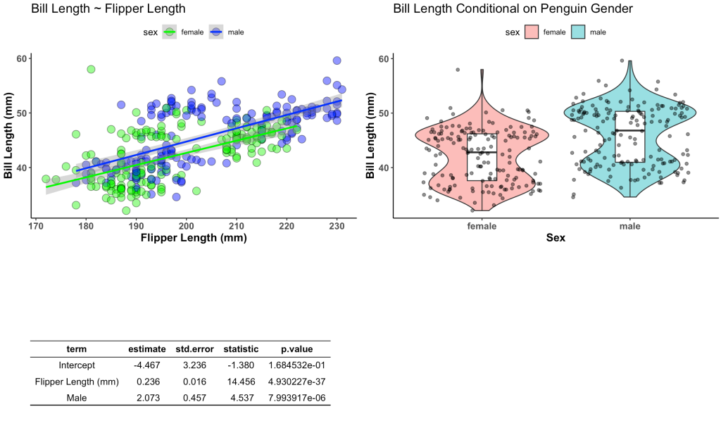
Recall that yesterday we constructed the below plot using both ggarrange() and the {patchwork} package.
I’m going to use both approaches and add a title and a bullet point caption box in the bottom right.
Titles & Captions with ggarrange()
I wont rehash all of the code from yesterday, but the ggarrange() table that we created with was constructed with the following code.
## Build table into a nice ggtextable() to visualize it
tbl <- ggtexttable(fit, rows = NULL, theme = ttheme("blank")) %>%
  tab_add_hline(at.row = 1:2, row.side = "top", linewidth = 2) %>%
  tab_add_hline(at.row = 4, row.side = "bottom", linewidth = 3, linetype = 1)
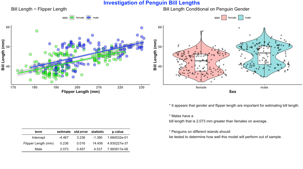
To create a bullet point caption box I need to first create a string of text that I want to display, using the paste() function. I then wrap this text into the ggparagraph() function so that it can be appropriately displayed on the plot. Then, similar to yesterday, I use the ggarrange() function to put the two plots, the table, and the caption box, into a single canvas.
## Create text for a caption
text <- paste("* It appears that gender and flipper length are important for estimating bill length.",
              " ",
              "* Males have a bill length that is 2.073 mm greater than females on average.",
              " ",
              "* Penguins on different islands should be tested to determine how well this model will perform out of sample.",
              sep = "\n")

text.p <- ggparagraph(text = text,
                      #face = "italic",
                      size = 12,
                      color = "black") +
  theme(plot.margin = unit(c(t = 1, b = -3, r = 1, l = 2),"cm"))


## Plots & Table together with the caption using ggarange()
final_display <- ggarrange(plt1, plt2, tbl, text.p,
          ncol = 2, nrow = 2)
I saved the canvas as final_display which I can now wrap in the annotate_figure() function to add the common title to the report.
## add a common title
annotate_figure(final_display, top = text_grob("Investigation of Penguin Bill Lengths",
                                      color = "blue", face = "bold", size = 18))
The finished product looks like this:
Titles & Captions with patchwork
Now, we will do the same thing with {patchwork}. Just like yesterday, to use {patchwork} we need to change the table from a ggtextable to a tableGrob. After that we can wrap it together with our two plots.
# Need to build the table as a tableGrob() instead of ggtextable
# to make it work with patch work
tbl2 <- tableGrob(fit, rows = NULL, theme = ttheme("blank")) %>%
  tab_add_hline(at.row = 1:2, row.side = "top", linewidth = 2) %>%
  tab_add_hline(at.row = 4, row.side = "bottom", linewidth = 3, linetype = 1)

# now visualize together
final_display2 <- wrap_plots(plt1, plt2, tbl2,
           ncol = 2,
           nrow = 2)
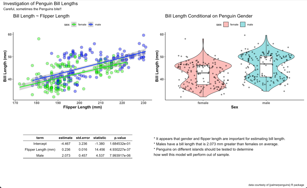
We stored the final canvas in the element final_display2. We can add a title, subtitle, caption, and bullet point box to this using patchwork’s plot_annotation() function by simply specifying the text that we would like.
final_display2 + plot_annotation(
  title = "Investigation of Penguin Bill Lengths",
  subtitle = "Careful, sometimes the Penguins bite!!",
  caption = "data courtesty of {palmerpenguins} R package") +
  grid::textGrob(hjust = 0, x = 0,
                   "* It appears that gender and flipper length are important for estimating bill length.\n* Males have a bill length that is 2.073 mm greater than females on average.\n* Penguins on different islands should be tested to determine\nhow well this model will perform out of sample.")
Ads here is our final report:
Wrapping up
There are two simple ways using two different R packages to create single page reports with plots, data tables, and even bullet point notes for the reader. Happy report constructing!
For the complete code to the blog article check out my GITHUB page.


