
In Part 1 of this series we were looking at data from a fake study, which evaluated the improvement in strength scores for two groups — Group 1 was a control group that received a normal training program and Group 2, the experimental group that received a special training program, designed to improve strength. In that first part we used a traditional t-test (frequentist) approach and a Bayesian approach, where we took advantage of a normal conjugate distribution. In order to use the normal-normal conjugate, we needed to make an assumption about a known population standard deviation. By using a known standard deviation it meant that we only needed to perform Bayesian updating for the mean of the distribution, allowing us to compare between group means and their corresponding standard errors. The problem with this approach is that we might not always have a known standard deviation to apply, thus we would want to be able to estimate this along with the mean — we need to estimate both parameters jointly!
Both Part 1 and Part 2 are available in a single file Rmarkdown file on my GitHub page.
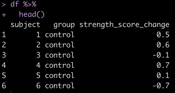
Let’s take a look at the first few rows of the data to help remind ourselves what it looked like.
Linear Regression
To estimate the joint distribution of the mean and standard deviation under the Bayesian framework we will work with a regression model where group (control or experimental) is the independent variable and the dependent variable is the change in strength score. We can do this because, recall, t-tests are really just regression underneath.
Let’s look at the output of a frequentist linear regression before trying a Bayesian regression.
fit_lm <- lm(strength_score_change ~ group, data = df)
summary(fit_lm)
confint(fit_lm)
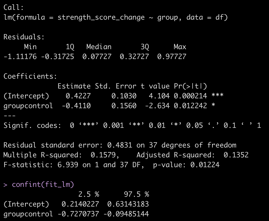
As expected, the results that we get here are the same as those that we previously obtained from our t-test in Part 1. The coefficient for the control group (-0.411) represents the difference in the mean strength score compared to the experimental group, whose mean change in strength score is accounted for in the intercept.
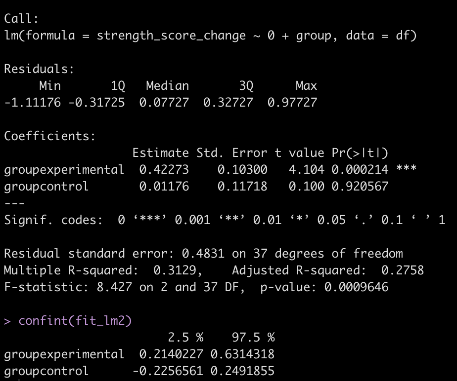
Because the experimental group is now represented as the model intercept, we can instead code the model without an intercept and get a mean change in strength score for both groups. This is accomplished by adding a “0” to the right side of the equation, telling R that we don’t want a model intercept.
fit_lm2 <- lm(strength_score_change ~ 0 + group, data = df)
summary(fit_lm2)
confint(fit_lm2)
Bayesian Regression
Okay, now let’s move into the Bayesian framework. We’ll utilize the help of the brilliant {brms} package, which compiles C++ and runs the Stan language under the hood, allowing you to use the simple and friendly R syntax that you’re used to.
Let’s start with a simple Bayesian Regression Model.
library(brms)

# Set 3 cores for parallel processing (helps with speed)
fit_bayes1 <- brm(strength_score_change ~ group,
                 data = df,
                 cores = 3,
                 seed = 7849
                 )

summary(fit_bayes1)

The output here is a little more extensive than what we are used to with the normal regression output. Let’s make some notes:
- The control group coefficient still represents the mean difference in strength score compared to the experimental group.
- The experimental groups mean strength score is still the intercept
- The coefficients for the intercept and control group are the same that we obtained with the normal regression.
- We have a new parameter at the bottom, sigma, which is a value of 0.50. This value represents the shared standard deviation between the two groups. If you recall the output of our frequentist regression model, we had a value called residual standard error, which was 0.48 (pretty similar). The one thing to add with our sigma value here is, like the model coefficients, it has its own error estimate and 95% Credible Intervals (which we do not get from the original regression output).
Before going into posterior simulation, we have to note that we only got one sigma parameter. This is basically saying that the two groups in our model are sharing a standard deviation. This is similar to running a t-test with equal variances (NOTE: the default in R’s t-test() function is “var.equal = FALSE”, which is usually a safe assumption to make). To specify a sigma value for both groups we will wrap the equation in the bf() function, which is a function for specifying {brms} formulas. In there, we will indicate different sigma values for each group to be estimated. Additionally, to get a coefficient for both groups (versus the experimental group being the intercept), we will add a “0″ to the right side of the equation, similar to what we did in our second frequentist regression model above.
group_equation <- bf(strength_score_change ~ 0 + group,
                     sigma ~ 0 + group)

fit_bayes2 <- brm(group_equation,
                 data = df,
                 cores = 3,
                 seed = 7849
                 )

summary(fit_bayes2)

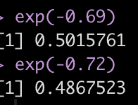
Now we have an estimate for each group (their mean change in strength score from pre to post testing) and a sigma value for each group (NOTE: To get this value to the normal scale we need to take is exponential as they are on a log scale, as indicated by the links statement at the top of the model output, sigma = log.). Additionally, we have credible intervals around the coefficients and sigmas.
exp(-0.69)
exp(-0.72)
We have not specified any priors yet, so we are just using the default priors. Before we try and specify any priors, let’s get posterior samples from our model (don’t forget to exponentiate the sigma values). We will also calculate a Cohen’s d as a measure of standardized effect.
Cohen’s d = (group_diff) / sqrt((group1_sd^2 + group2_sd^2) / 2)
bayes2_draws <- as_draws_df(fit_bayes2) %>%
  mutate(across(.cols = contains("sigma"),
                ~exp(.x)),
         group_diff = b_groupexperimental - b_groupcontrol,
         cohens_d = group_diff / sqrt((b_sigma_groupexperimental^2 + b_sigma_groupcontrol^2)/2))

bayes2_draws %>%
  head()

Let’s make a plot of the difference in means and Cohen’s d across our 4000 posterior samples.
par(mfrow = c(1,2))
hist(bayes2_draws$group_diff,
main = "Posterior Draw of Group Differences",
xlab = "Group Differences")
abline(v = 0,
col = "red",
lwd = 3,
lty = 2)
hist(bayes2_draws$cohens_d,
main = "Posterior Draw of Cohen's d",
xlab = "Cohen's d")

Adding Priors
Okay, now let’s add some priors and repeat the process of plotting the posterior samples. We will use the same normal prior for the means that we used in Part 1, Normal(0.1, 0.3) and for the sigma value we will use a Cauchy prior, Cauchy(0, 1).
## fit model
fit_bayes3 <- brm(group_equation,
                 data = df,
                 prior = c(
                       set_prior("normal(0.1, 0.3)", class = "b"),
                       set_prior("cauchy(0, 1)", class = "b", dpar = "sigma")
                 ),
                 cores = 3,
                 seed = 7849
                 )

summary(fit_bayes3)

## exponent of the sigma values
exp(-0.66)
exp(-0.70)

## posterior draws
bayes3_draws <- as_draws_df(fit_bayes3) %>%
  mutate(across(.cols = contains("sigma"),
                ~exp(.x)),
         group_diff = b_groupexperimental - b_groupcontrol,
         cohens_d = group_diff / sqrt((b_sigma_groupexperimental^2 + b_sigma_groupcontrol^2)/2))

bayes3_draws %>%
  head()

## plot sample of group differences and Cohen's d
par(mfrow = c(1,2))
hist(bayes3_draws$group_diff,
     main = "Posterior Draw of Group Differences",
     xlab = "Group Differences")
abline(v = 0,
       col = "red",
       lwd = 3,
       lty = 2)
hist(bayes3_draws$cohens_d,
     main = "Posterior Draw of Cohen's d",
     xlab = "Cohen's d")

Combine all the outputs together
Combine all of the results together so we can evaluate what has happened.
no_prior_sim_control_mu <- mean(bayes2_draws$b_groupcontrol)
no_prior_sim_experimental_mu <- mean(bayes2_draws$b_groupexperimental)
no_prior_sim_diff_mu <- mean(bayes2_draws$group_diff)

no_prior_sim_control_sd <- sd(bayes2_draws$b_groupcontrol)
no_prior_sim_experimental_sd <- sd(bayes2_draws$b_groupexperimental)
no_prior_sim_diff_sd <- sd(bayes2_draws$group_diff)

with_prior_sim_control_mu <- mean(bayes3_draws$b_groupcontrol)
with_prior_sim_experimental_mu <- mean(bayes3_draws$b_groupexperimental)
with_prior_sim_diff_mu <- mean(bayes3_draws$group_diff)

with_prior_sim_control_sd <- sd(bayes3_draws$b_groupcontrol)
with_prior_sim_experimental_sd <- sd(bayes3_draws$b_groupexperimental)
with_prior_sim_diff_sd &<- sd(bayes3_draws$group_diff)

data.frame(group = c("control", "experimental", "difference"), observed_avg = c(control_mu, experimental_mu, t_test_diff), posterior_sim_avg = c(posterior_mu_control, posterior_mu_experimental, mu_diff), no_prior_sim_avg = c(no_prior_sim_control_mu, no_prior_sim_experimental_mu, no_prior_sim_diff_mu), with_prior_sim_avg = c(with_prior_sim_control_mu, with_prior_sim_experimental_mu, with_prior_sim_diff_mu), observed_standard_error = c(control_sd / sqrt(control_N), experimental_sd / sqrt(experimental_N), se_diff), posterior_sim_standard_error = c(posterior_sd_control, posterior_sd_experimental, sd_diff), no_prior_sim_standard_error = c(no_prior_sim_control_sd, no_prior_sim_experimental_sd, no_prior_sim_diff_sd), with_prior_sim_standard_error = c(with_prior_sim_control_sd, with_prior_sim_experimental_sd, with_prior_sim_diff_sd) ) %>%
  mutate(across(.cols = -group,
                ~round(.x, 3))) %>%
  t() %>%
  as.data.frame() %>%
  setNames(., c("Control", "Experimental", "Difference")) %>%
  slice(-1) %>%
  mutate(models = rownames(.),
    group = c("Average", "Average", "Average", "Average", "Standard Error", "Standard Error", "Standard Error", "Standard Error")) %>%
  relocate(models, .before = Control) %>%
  group_by(group) %>%
  gt::gt()

Let’s make some notes:
- First, observed refers to the actual observed data, posterior_sim is our normal-normal conjugate (using a known standard deviation), no_prior_sim is our Bayesian regression with default priors and with_prior_sim is our Bayesian regression with pre-specified priors.
- In the normal-normal conjugate (posterior_sim) analysis (Part 1), both the control and experimental groups saw their mean values get pulled closer to the prior leading to a smaller between group difference than we saw in the observed data.
- The Bayesian regression with no priors specified (no_prior_sim) resulted in a mean difference that is pretty much identical to the outcome we saw with our t-test on the observed data.
- The Bayesian Regression with specified priors (with_prior_sim) ends up being somewhere in the middle of the observe data/Bayes Regression with no priors and the normal-normal conjugate. The means for both groups are pulled close to the prior but not as much as the normal-normal conjugate means (posterior_sim). Therefore, the mean difference between groups is higher than the posterior_sim output but not as large as the observed data (because it is influenced by our prior). Additionally, the group standard errors are more similar to the observed data with the Bayesian regression with priors than the Bayesian regression without priors and the normal-normal Bayesian analysis.
Wrapping Up
We’ve gone over a few approaches to comparing two groups using both Frequentist and Bayesian frameworks. Hopefully working through the analysis in this way provides an appreciation for both frameworks. If we have prior knowledge, which we often do, it may help to code it directly into our analysis and utilize a Bayesian approach that helps us update our present beliefs about a phenomenon or treatment effect.
Both Part 1 and Part 2 are in a single file on my GitHub page.
If you notice any errors or issues feel free to reach out via email!