Introduction
A colleague had asked me if I knew of a way to obtain model fit metrics, such as AIC or r-squared, from the optim() function. First, optim() provides a general-purpose method of optimizing an algorithm to identify the best weights for either minimizing or maximizing whatever success metric you are comparing your model to (e.g., sum of squared error, maximum likelihood, etc.). From there, it continues until the model coefficients are optimal for the data.
To make optim() work for us, we need to code the aspects of the model we are interested in optimizing (e.g., the regression coefficients) as well as code a function that calculates the output we are comparing the results to (e.g., sum of squared error).
Before we get to model fit metrics, let’s walk through how optim() works by comparing our results to a simple linear regression. I’ll admit, optim() can be a little hard to wrap your head around (at least for me, it was), but building up a simple example can help us understand the power of this function and how we can use it later on down the road in more complicated analysis.
Data
We will use data from the Lahman baseball data base. I’ll stick with all years from 2006 on and retain only players with a minimum of 250 at bats per season.
library(Lahman)
library(tidyverse)

data(Batting)

df <- Batting %>%
  filter(yearID >= 2006,
         AB >= 250)

head(df)
Linear Regression
First, let’s just write a linear regression to predict HR from Hits, so that we have something to compare our optim() function against.
fit_lm <- lm(HR ~ H, data = df)
summary(fit_lm)

plot(df$H, df$HR, pch = 19, col = "light grey")
abline(fit_lm, col = "red", lwd = 2)
The above model is a simple linear regression model that fits a line of best fit based on the squared error of predictions to the actual values.
(NOTE: We can see from the plot that this relationship is not really linear, but it will be okay for our purposes of discussion here.)
We can also use an optimizer to solve this.
Optimizer
To write an optimizer, we need two functions:
- A function that allow us to model the relationship between HR and H and identify the optimal coefficients for the intercept and the slope that will help us minimize the residual between the actual and predicted values.
- A function that helps us keep track of the error between actual and predicted values as optim() runs through various iterations, attempting a number of possible coefficients for the slope and intercept.
Function 1: A linear function to predict HR from hits
hr_from_h <- function(H, a, b){
  return(a + b*H)
}
This simple function is just a linear equation and takes the values of our independent variable (H) and a value for the intercept (a) and slope (b). Although, we can plug in numbers and use the function right now, the values of a and b have not been optimized yet. Thus, the model will return a weird prediction for HR. Still, we can plug in some values to see how it works. For example, what if the person has 30 hits.
hr_from_h(H = 30, a = 1, b = 1)
Not a really good prediction of home runs!
Function 2: Sum of Squared Error Function
Optimizers will try and identify the key weights in the function by either maximizing or minimizing some value. Since we are using a linear model, it makes sense to try and minimize the sum of the squared error.
The function will take 3 inputs:
- A data set of our dependent and independent variables
- A value for our intercept (a)
- A value for the slope of our model (b)
sum_sq_error <- function(df, a, b){

  # make predictions for HR
  predictions <- with(df, hr_from_h(H, a, b))

  # get model errors
  errors <- with(df, HR - predictions)

  # return the sum of squared errors
  return(sum(errors^2))

}
Let’s make a fake data set of a few values of H and HR and then assign some weights for a and b to see if the sum_sq_error() produces a single sum of squared error value.
fake_df <- data.frame(H = c(35, 40, 55),
                        HR = c(4, 10, 12))

sum_sq_error(fake_df,
             a = 3,
             b = 1)
It worked! Now let’s write an optimization function to try and find the ideal weights for a and b that minimize that sum of squared error. One way to do this is to create a large grid of values, write a for loop and let R plug along, trying each value, and then find the optimal values that minimize the sum of squared error. The issue with this is that if you have models with more independent variables, it will take really long. A more efficient way is to write an optimizer that can take care of this for us.
We will use the optim() function from base R.
The optim() function takes 2 inputs:
- A numeric vector of starting points for the parameters you are trying to optimize. These can be any values.
- A function that will receive the vector of starting points. This function will contain all of the parameters that we want to optimize. This function will take our sum_sq_error() function and it will get passed the starting values for a and b and then find their values that minimize the sum of squared error.
optimizer_results <- optim(par = c(0, 0),
                           fn = function(x){
                             sum_sq_error(df, x[1], x[2])
                             }
                           )
Let’s have a look at the results.
In the output:
- value tells us the sum of the squared error
- par tells us the weighting for a (intercept) and b (slope)
- counts tells us how many times the optimizer ran the function. The gradient is NA here because we didn’t specify a gradient argument in our optimizer
- convergence tells us if the optimizer found the optimal values (when it goes to 0, that means everything worked out)
- message is any message that R needs to inform us about when running the optimizer
Let’s focus on par and value since those are the two values we really want to know about.
First, notice how the values for a and b are nearly the exact same values we got from our linear regression.
a_optim_weight <- optimizer_results$par[1]
b_optim_weight <- optimizer_results$par[2]

a_reg_coef <- fit_lm$coef[1]
b_reg_coef <- fit_lm$coef[2]

a_optim_weight
a_reg_coef

b_optim_weight
b_reg_coef
Next, we can see that the sum of squared error from the optimizer is the same as the sum of squared error from the linear regression.
sse_optim <- optimizer_results$value
sse_reg <- sum(fit_lm$residuals^2)

sse_optim
sse_reg
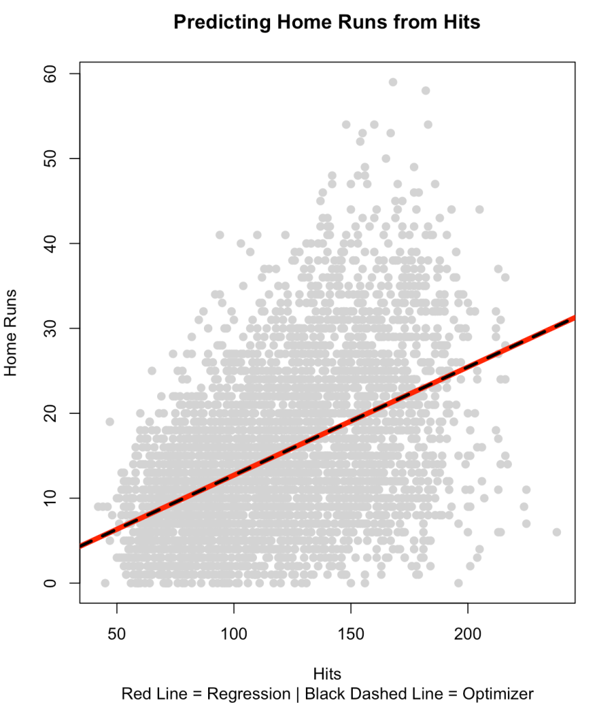
We can finish by plotting the two regression lines over the data and show that they produce the same fit.
plot(df$H,
     df$HR,
     col = "light grey",
     pch = 19,
     xlab = "Hits",
     ylab = "Home Runs")
title(main = "Predicting Home Runs from Hits",
     sub = "Red Line = Regression | Black Dashed Line = Optimizer")
abline(fit_lm, col = "red", lwd = 5)
abline(a = a_optim_weight,
       b = b_optim_weight,
       lty = 2,
       lwd = 3,
       col = "black")
Model Fit Metrics
The value parameter from our optimizer output returned the sum of squared error. What if we wanted to return a model fit metric, such as AIC or r-squared, so that we can compare several models later on?
Instead of using the sum of squared errors function, we can attempt to minimize AIC by writing our own AIC function.
aic_func <- function(df, a, b){

  # make predictions for HR
  predictions <- with(df, hr_from_h(H, a, b))

  # get model errors
  errors <- with(df, HR - predictions)

  # calculate AIC
  aic <- nrow(df)*(log(2*pi)+1+log((sum(errors^2)/nrow(df)))) + ((length(c(a, b))+1)*2)
  return(aic)

}
We can try out the new function on the fake data set we created above.
aic_func(fake_df,
             a = 3,
             b = 1)
Now, let’s run the optimizer with the AIC function instead of the sum of square error function.
optimizer_results <- optim(par = c(0, 0),
                           fn = function(x){
                             aic_func(df, x[1], x[2])
                             }
                           )

optimizer_results
We get the same coefficients with the difference being that the value parameter now returns AIC. We can check that this AIC compares to our original linear model.
AIC(fit_lm)
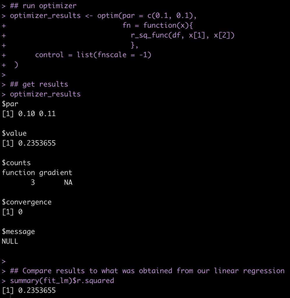
If we instead wanted to obtain an r-squared, we can write an r-squared function. In the optimizer, since a higher r-squared is better, we need to indicate that we are wanting to maximize this value (optim defaluts to minimization). To do this we set the fnscale argument to -1. The only issue I have with this function is that it doesn’t return the coefficients properly in the par section of the results. Not sure what is going on here but if anyone has any ideas, please reach out. I am able to produce the exact result of r-squared from the linear model, however.
## r-squared function
r_sq_func <- function(df, a, b){

  # make predictions for HR
  predictions <- with(df, hr_from_h(H, a, b))

  # r-squared between predicted and actual HR values
  r2 <- cor(predictions, df$HR)^2
  return(r2)

}

## run optimizer
optimizer_results <- optim(par = c(0.1, 0.1),
                           fn = function(x){
                             r_sq_func(df, x[1], x[2])
                             },
      control = list(fnscale = -1)
 )

## get results
optimizer_results

## Compare results to what was obtained from our linear regression
summary(fit_lm)$r.squared
Wrapping up
That was a short tutorial on writing an optimizer in R. There is a lot going on with these types of functions and they can get pretty complicated very quickly. I find that starting with a simple example and building from there is always useful. We additionally looked at having the optimizer return us various model fit metrics.
If you notice any errors in the code, please reach out!
Access to the full code is available on my GitHub page.


