In yesterday’s post, I offered an approach to using {tidymodes} when you don’t want to split your data into training and testing sets, but rather, you want to fit all of your data using cross-validated folds and then save the model and deploy it later on with new data sets. Recall that the reason you’d want to do this is because you might not have enough data where you feel good about removing some of it for a testing set, ultimately decreasing the number of observations your model can learn from.
After that post, I got an email from someone asking how they could save the entire workflow for later deployment as yesterday’s article only saved the model fit following cross-validation. Storing the workflow can be critical when you have a data and.or a model that requires various preprocessing steps prior to making forecasts. One of the advantages of the {tidymodels} framework is the ability to combine the preprocessing tasks in one step and then fit the model all at once. This keeps your script nice and tidy and makes it easy to see what is taking place at each step.
The issue we have when working with just the cross-validated folds is that you aren’t fitting the model to a training/testing split of data once you are done fitting it. In most {tidymodels} examples, model fitting is done with the last_fit() function, which requires a split data set, which was generated via the initial_split() function. Form there you can extract the workflow and save it for later deployment. Consequently, there are a few extra steps to make this work smoothly when saving a model that was fit using only cross-validated folds.
So, to follow up on yesterday, I’ll walk through a random forest classification example where I’ll fit a model to cross-validation folds of the mtcars data set, I’ll save the entire recipe (where preprocessing takes place), I’ll save the model, and then I’ll show how you can use both the saved recipe and model to make predictions on a new data set. Additionally, to make things more interesting, I will tune the random forest model and show how to extract the tuned parameters and re-fit the model before saving it.
Load packages & data
### get data
df <- mtcars
head(df)
table(df$cyl)

df$cyl <- as.factor(df$cyl)
Create cross-validated folds & specify a random forest classifier
### specify random forest model
rf_spec_with_tuning <-rand_forest(mtry = tune(), trees = tune()) %>%
  set_engine("randomForest", importance = TRUE) %>%
  set_mode("classification")
Build a tuning grid
We will allow {tidymodels} to optimize both mtry and the trees.
### build a tuning grid
rf_tune_grid <- grid_regular(
  mtry(range = c(1, 10)),
  trees(range = c(500, 800)),
  levels = 5
)
Create the model recipe
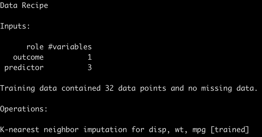
The mtcars data set is complete and has no missing values. But, that doesn’t mean that future data that we will be deploying the model on will be free from missing values. So, to be sure that we can handle this in the future, if we need to, I’m going to create an imputation step in the recipe that will use k-nearest neighbor, which will you the 3 nearest neighbors, to impute any NA values of the independent variables.
NOTE: I’m not saying this is the best imputation approach here. I’m simply creating an additional step in the model recipe that can be deployed later to show how it works.
### recipe -- set up imputation for new data that might have missing values
cyl_rec <- recipe(cyl ~ mpg + disp + wt, data = df) %>%
  step_impute_knn(mpg, disp, wt,
                  neighbors = 3)
Set up the workflow
Combine the preprocessing recipe and the random forest model, which still needs to be tuned, into a single workflow.
### workflow
cyl_wf <- workflow() %>%
  add_recipe(cyl_rec) %>%
  add_model(rf_spec_with_tuning)
Set up a control function for storing the model predictions on the cross-validated folds
### set a control function to save the predictions from the model fit to the CV-folds
ctrl <- control_resamples(save_pred = TRUE)
Tune the model parameters during the model fitting process
### fit model
cyl_tune <- tune_grid(
  cyl_wf,
  resamples = df_cv,
  grid = rf_tune_grid,
  control = ctrl
)
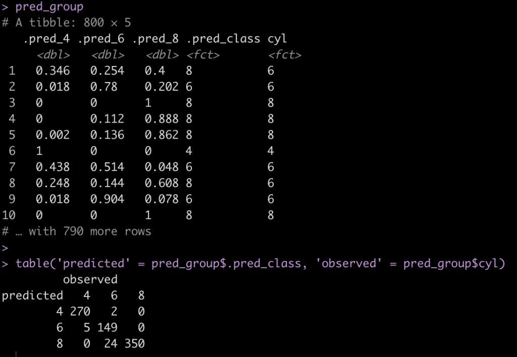
Get the model predictions from the cross-validated tunning
### get predictions
pred_group <- cyl_tune %>%
  unnest(cols = .predictions) %>%
  select(.pred_4, .pred_6, .pred_8, .pred_class, cyl)

pred_group

table('predicted' = pred_group$.pred_class, 'observed' = pred_group$cyl)
Get the optimized values for mtry and trees
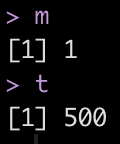
After tuning the model, we want to get the mtry and trees parameters that produced the best ROC/AUC, so we will pull those values out of our tuning grid, cyl_tune. In this instance, an mtry of 1 and 500 trees appear to be the optimal values.
NOTE: We could have extracted the mtry and trees parameters that optimized model accuracy instead.
# get the optimized numbers for mtry and trees
m <- select_best(cyl_tune, "roc_auc") %>% pull(mtry)
t <- select_best(cyl_tune, "roc_auc") %>% pull(trees)

m
t
Re-specify the model and re-fit the workflow
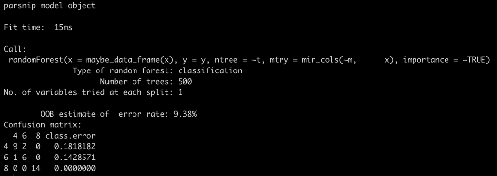
Since we are working with cross-validated samples and not a training/testing set, we can’t just fit the last or fit the best model because this isn’t split data. To get the optimal model we need to actual re-specify the random forest model with the mtry and trees values we extracted above. So re-fit a new workflow with the optiized mtry and trees parameters to ensure that the tuned model is used for our final model fit.
# re-specify the model with the optimized values
rf_spec_tuned <-rand_forest(mtry = m, trees = t) %>%
  set_engine("randomForest", importance = TRUE) %>%
  set_mode("classification")

# re-set workflow
cyl_wf_tuned <- workflow() %>%
  add_recipe(cyl_rec) %>%
  add_model(rf_spec_tuned)
Extract & save the final recipe
Now that the tuned model has been fit we will need to extract the final recipe and then save it as an .RDA file so that we can load it for deployment later on. To do this, we use the extract_recipe() function after fitting the tuned model to our original data set.
# extract the final recipe for pre-processing of new data
cyl_final_rec <- cyl_wf_tuned %>%
  fit(df) %>%
  extract_recipe()

save(cyl_final_rec, file = "cyl_final_rec.rda")
load("cyl_final_rec.rda")
cyl_final_rec
Extract & save the final model fit
Once we have the recipe, which holds all of our preprocessing steps, we then need to extract the actual model fit so that we can make future predictions on new data.
# extract final model
cyl_final_tuned <- cyl_wf_tuned %>%
  fit(df) %>%
  extract_fit_parsnip()

save(cyl_final_tuned, file = "cyl_final_tuned.rda")
load("cyl_final_tuned.rda")

cyl_final_tuned
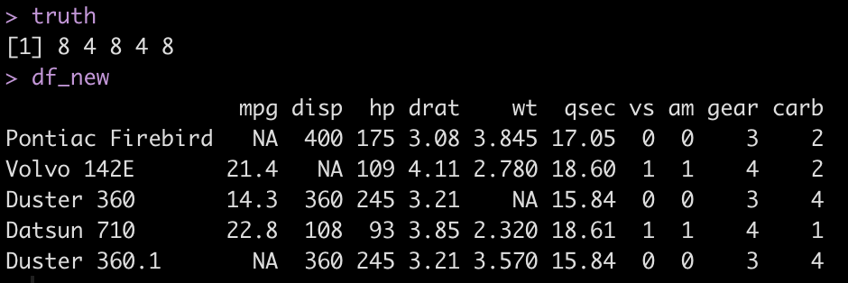
Create a new data set and add missing values to some of the independent variables
Now that our recipe and model fit are saved we will create some new data and add some missing values to show how the impute function, which we created in the recipe, works.
We will also save the cyl value for this new data (the truth) so we can check our work once the model predictions are done. Prior to making predictions on this new data we will drop the cyl column from this new data set to make it look more realistic to what we would see in the real world (IE, we’d never have the actual output we are trying to forecast).
### Create New Data with NAs
set.seed(947)
row_ids <- sample(x = 1:nrow(mtcars), size = 5, replace = TRUE)

df_new <-mtcars[row_ids, ]
df_new[2, 3] <- NA
df_new[c(1,5), 1] <- NA
df_new[3, 6] <- NA

# get the actual cyl values for this new data
truth <- df_new$cyl
truth

# drop the cyl column to pretend like this is new data
df_new$cyl <- NULL
df_new
Apply the recipe to the new data
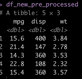
Notice that we have some NAs in a few of the predictor columns (mpg, disp, and wt). We apply the recipe to the new data set by using the bake() function to impute those values using information about the data that was gained during the model workflow that we build back when we fit the model.
### Apply the pre-processing recipe to the new data
df_new_pre_processed <- cyl_final_rec %>%
  bake(new_data = df_new)

df_new_pre_processed
Make the final predictions using the saved model
Now that we have imputed NAs using the recipe we are ready to make cyl predictions on the new data. After making predictions we will combine the predicted class and the probability of each of the three classes with the new data set.
### Make a prediction for cyl
pred_cyl <- predict(cyl_final_tuned, new_data = df_new_pre_processed, type = "class")
df_new_pre_processed <- cbind(df_new_pre_processed, pred_cyl)

### get probability of each class
pred_probs <- predict(cyl_final_tuned, new_data = df_new_pre_processed, type = "prob")
df_new_pre_processed <- cbind(df_new_pre_processed, pred_probs)
df_new_pre_processed
See how well the model predicted on this new data, even after having to impute some values for each observation.
table('predicted' = df_new_pre_processed$.pred_class, 'actual' = truth)
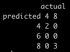
The model predicted all 5 new observations correctly.
And that’s it! Those are the steps to follow for using all of your data to fit and tune a model with cross-validated folds, save the preprocessing steps and tuned model, and then apply it to a new set of observations.
All of the code for this blog article is available on my GITHUB page.

