Category Archives: Bayesian Model Building

First time collecting new data on your team? Bayesian updating can help!

A few weeks ago I was speaking with some athletic trainers and strength coaches who work for a university football team. They asked me the following question:

“We are about to start using GPS to collect data on our team. But we have never collected anything in the past. How do we even start to understand whether the training sessions we are doing are normal or not? Do we need to tell the coach that we have to collect data for a full season before we know anything meaningful?”

This is a fascinating question and it is an issue that we all face at some point in the applied setting. Whenever we start with a new data collection method or a new technology it can be daunting to think about how many observations we need in order to start making sense of our data and establishing what is “normal”.

We always have some knowledge!

My initial reaction to the question was, “Why do you believe that you have NOTHING to make a decision on?”

Sure, you currently have no data on your specific team, but that doesn’t mean that you have no prior knowledge or expectations! This is where Bayes can help us out. We can begin collecting data on day 1, combine it with our prior knowledge, and continually update our knowledge until we get to a point where we have enough data on our own team that we no longer need the prior.

Where does our prior knowledge come from?

Establishing the prior in this case can be done in two ways:

  1. Get some video of practices, sit there and watch a few players in each position group and record, to the best you can estimate, the amount of distance they covered for each rep they perform in each training drill.
  2. Pull some of the prior research on college football and try and make a logical estimation of what you’d assume a college football practice to be with respect to various training metrics (total distance, sprints, high speed running, accelerations, etc).

Option 1 is a little time consuming (though you probably wont need to do as many practices as you think) and probably not the option most people want to hear (Side Note, I’ve done this before and, yes, it does take some time but you learn a good deal about practice by manually notating it. When trying to do total distance always remember that if a WR runs a route they have to always run back to the line of scrimmage once the play is over, so factor that into the distance covered in practice).

Option 2 is reasonably simple. Off the top of my head, the two papers that could be useful here are from DeMartini et al (2011) and Wellman et al (2016). The former quantifies training demands in collegiate football practices while the latter is specific to the quantification of competitive demands during games. To keep things brief for the purposes of this blog post, I’ll stick to total distance. I’ve summarized the findings from these papers in the table below.

Notice that the DeMartini paper uses a broader position classification — Linemen or Non-Linemen. As such, it is important to consider that the mean’s and standard deviations might be influenced by the different ergonomic demands of the groups that have been pooled together. Also, DeMartini’s paper is of practice demands, so the overall total distance may differ compared to what we would see in games, which is what Wellman’s data is showing us. All that aside, we can still use this information to get a general sense for a prior.

Let’s bin the players into groups that compete against each other and therefore share some level of physical attributes.

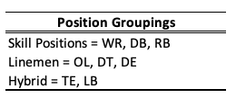
Rather than getting overly complicated with Markov Chain Monte Carlo, will use normal-normal conjugate (which we discussed in TidyX 102). This approach provides us a with simple shortcut for performing Bayesian inference when dealing with data coming from a normal distribution. To make this approach work, we need three pieces of prior information from our data:

  1. A prior mean (prior mu)
  2. A prior standard deviation for the mean (sigma) which we will convert to precision (1 / sigma^2)
  3. An assumed/known standard deviation for the data

The first two are rather easy to wrap our heads around. We need to establish a reasonable prior estimate for the average total distance and some measure of variability around that mean. The third piece of information is the standard deviation of the data and we need to assume that it is known and fixed.

We are dealing with a Normal distribution, which is a two parameter distribution, possessing a Mean and Standard Deviation. Both of these parameters have variability around them (they have their own measures of center and dispersion). The Mean is what we are trying to figure out for our team, so we set a prior center (mu) and dispersion (sigma) around it. Because we are stating up front that the Standard Deviation for the population is known, we are not concerned with the dispersion around that variable (if we don’t want to make this assumption we will need to resort to an approach that allows us to determine both of these parameters, such as GIBBS sampling).

Setting Priors

Let’s stick with the Skill Positions for the rest of this article. We can take an average of the WR, DB, and RB distances to get a prior mean. The dispersion around this mean is tricky and Wellman’s paper only tells us the total number of athletes in their sample, not the number of athletes per position. From the table above we see that the WR group has a standard deviation of 996. We will make the assumption that there were 5 WR’s that were tracked and thus the standard error of the mean (the dispersion around the mean) ends up being 996 / sqrt(5) = 445. Since we also have DB’s and RB’s in our skill grouping lets just round that up to 500. Finally, just eyeballing the standard deviations in the table above, I set the known SD for the population of skill positions to be 750. My priors for all three of our position groups are as follows:

Bayesian Updating

Looking at the Skill Positions, what we want to do is observe each training session for our team and update our prior knowledge about the normal amount of total running distance we expect skill position players to do given what we know.

First, let’s specify our priors and then create a table of 10 training sessions that we’ve collected on our team. I’ve also created a column that provides a running/cumulative total distance for all of the sessions as we will need this for our normal-normal conjugate equation.

library(tidyverse)

## set a prior for the mean
mu_prior <- 4455
mu_sd <- 500
tau_prior <- 1/mu_sd^2

## To use the normal-normal conjugate we will make an assumption that the standard deviation is "known"
assumed_sd <- 750
assumed_tau <- 1 / assumed_sd^2

## Create a data frame of observations
df <- data.frame(
  training_day = 1:10,
  dist = c(3800, 3250, 3900, 3883, 3650, 3132, 3300, 3705, 3121, 3500)
)

## create a running/cumulative sum of the outcome of interest
df <- df %>%
  mutate(total_dist = cumsum(dist))

df


We discussed the equation for updating our prior mean in TidyX 102. We will convert the standard deviations to precision (1/sd^2) for the equations below. The equation for updating our knowledge about the average running distance in practice for our skill players is as follows:


Because we want to do this in-line, we will want to update our knowledge about our team’s training after every training sessions. As such, the mu_prior and tau_prior will be updated with the row above them and session 1 will be updated with the initial priors. To make this work, we will program a for() loop in R which will update our priors after each new observation.

First, we create a few vectors to store our values. NOTE: The vectors need to be 1 row longer than the number of observations we have in the data set since we will be starting with priors before observing any data.

## Create a vector to store results from the normal-normal conjugate model
N <- length(df$dist) + 1
mu <- c(mu_prior, rep(NA, N - 1))
tau <- c(tau_prior, rep(NA, N - 1))
SD <- c(assumed_sd, rep(NA, N - 1))

Next, we are ready to run our for() loop and then put the output after each observation into the original data set (NOTE: remember to remove the first element of each output vector since it just contains our priors, before observing any data).

## For loop to continuously update the prior with every new observation
for(i in 2:N){

## Set up vectors for the variance, denominator, and newly observed values
numerator <- tau[i - 1] * mu[i - 1] + assumed_tau * df$total_dist[i - 1]
denominator <- tau[i - 1] + df$training_day[i - 1] * assumed_tau

mu[i] <- numerator / denominator
tau[i] <- denominator
SD[i] <- sqrt(1 / denominator)

}

df$mu_posterior <- round(mu[-1], 0)
df$SD_posterior <- round(SD[-1], 0)
df$tau_posterior <- tau[-1]

df

The final row in our data set represents the most up to date knowledge we have about our skill players average total running distance (mu_posterior = 3620 ± 99 yards) at practice. We can compare these results to summary statistics produced on the ten rows of our distance data:

### look at the summary stats after 10 sessions
mean(df$dist)            # Mean
sd(df$dist) / sqrt(10)   # Standard Error of the Mean
sd(df$dist)              # Standard Deviation

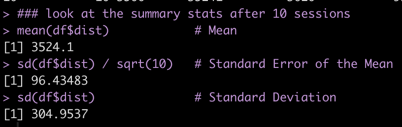
The posterior mean (mu_posterior) and posterior SD of the mean (SD_posterior) are relatively similar to what we have observed for our skill players after 10 training sessions (3524 with a standard error of 96). Our assumed SD was rather large to begin with (750) but the standard deviation for our skill players over the 10 observed sessions is much lower (305).

We’ve effectively started with prior knowledge of how much average total distance per training session we expect our skill players to perform and updated that knowledge, after each session, to learn as we go rather than waiting for enough data to begin having discussions with coaches.

Plot the data

Finally, let’s make a plot of the data to see what it looks like.

The grey shaded region shows the 95% confidence intervals around the posterior mean (red line) which are being updated after each training session. Notice that after about 8 sessions the data has nearly converged to something that is bespoke to our team’s skill players. The dashed line represents the average of our skill players’ total distance after 10 sessions. Note that we would not be able to compute this line until after the 10 sessions (for a team that practices 3 times a week, that would take 3 weeks!). Also note that taking a rolling average over such a short time period (e.g., a rolling average of every 3 or 4 sessions) wouldn’t have produced the amount of learning that we were able to obtain with the Bayesian updating approach.

Wrapping Up

After the first 3 sessions we’d be able to inform the coach that our skill players are performing less total running distance than what we initially believed skill players in college football would do, based on prior research. This is neither good nor bad — it just is. It may be more a reflection of the style of practice or the schematics that our coach employs compared to those of the teams that the original research is calculated on.

After about 6 sessions we are able to get a clearer picture of the running demands of our skill players and help the coach make a more informed decision about the total distance being performed by our skill players and hopefully assist with practice planning and weekly periodization. After about 9 or 10 sessions the Bayesian updating approach has pretty much converged with the nuances of our own team and we can begin to use our own data to make informed decisions.

Most importantly, we were able to update our knowledge about the running demands of our skill players, in real time, without waiting several weeks to figure out what training looks like for our team.

How much less running are our skill players doing compared to those of the players reported in the study?

This is a logical next question a coach might ask. For this we’d have to use a different type of Bayesian approach to compare what we are observing to our prior parameters and then estimate the magnitude of the difference. We will save this one for another blog post, though.

Finally, this Bayesian updating approach is not only useful when just starting to collect new data on your team. You can use priors from this season at the start of training camp next season to compare work rates to what you’d believe to be normal for your own team. You can also use this approach for the start of new training phases or for return to play, when a player begins a running program. Any time you start collecting new data on new people there is an opportunity to start out with your prior knowledge and beliefs and update as you go along. You always have some knowledge — usually more than you think!

All of the code for this article is available on my GITHUB page.

Confidence Intervals vs Prediction Intervals – A Frequentist & Bayesian Example

We often construct models for the purpose of estimating some future value or outcome. While point estimates for a forecasting future outcomes are interesting it is important to remember that the future contains a lot of uncertainty. As such, a reflection of this uncertainty is often conveyed using confidence intervals (which make a statement about the uncertainty of a population mean) or prediction intervals (which make a statement about a new/future observation for an individual within the population).

This tutorial will walk through how to calculate confidence intervals and prediction intervals by hand and then show the corresponding R functions for obtaining these values. We will finish by building the same model using a Bayesian framework and calculate the highest posterior density intervals and prediction intervals.

All of code is accessible through my GITHUB page.

Loading Packages & Data

We will use the Lahman baseball data set. For the purposes of this example, we will constrain our data to all MLB seasons after 2009 and players who had at least 250 At Bats in those seasons.

library(tidyverse)
library(broom)
library(Lahman)

theme_set(theme_minimal())

data(Batting)

df <- Batting %>%
  filter(yearID >= 2010,
         AB >= 250)


EDA

Let’s explore the relationship between Hits (H) and Runs Batted In (RBI) in our data set.


cor.test(df$H, df$RBI)

We see a very positive correlation suggesting that as a player gets more hits they tend to also have more RBI’s.

A Simple Regression Model

We will build a simple model that regresses RBI’s on Hits.

rbi_fit <- df %>%
  lm(RBI ~ H, data = .)

tidy(rbi_fit)
confint(rbi_fit)

  • Using tidy() from the broom package, we see that for every additional Hit we estimate a player to increase their RBI, on average, by 0.482.
  • We use the confint() function to produce the confidence intervals around the model coefficients.


Estimating Uncertainty

We can use the above model to forecast the expected number of RBI’s for a player given a number of hits.

For example, a player that has 100 hits would be estimated to produce approximately 49 RBI’s.


hits <- 100
pred_rbi <-  round(rbi_fit$coef[1] + rbi_fit$coef[2]*hits, 1)
pred_rbi

49 RBI’s is rather precise. There is always going to be some uncertainty around a number like this. For example, a player could be a good hitter but play on a team with poor hitters who don’t get on base thus limiting the possibility for all the hits he is getting to lead to RBI’s.

There are two types of questions we may choose to answer around our prediction:

  1. Predict the average RBI’s for players who get 100 hits.
  2. Predict the average RBI’s for a single player who gets 100 hits.

The point estimate, which we calculated above, will be the same for these two questions. Where they will differ is in the uncertainty we have around that estimate. Question 1 is a statement about the population (the average RBIs for all players who had 100 hits) while question 2 is a statement about an individual (the average RBI’s for a single player). Consequently, the confidence interval that we calculate to estimate our uncertainty for question 1 will be smaller than the prediction interval that we calculate to estimate our uncertainty for question 2.

Necessary Information for Computing Confidence Intervals & Prediction Intervals

In order to calculate the confidence interval and prediction interval by hand we need the following pieces of data:

  1. The model degrees of freedom.
  2. A t-critical value corresponding to the level of uncertainty we are interested in (here we will use 95%).
  3. The average number of hits (our independent variable) observed in our data.
  4. The standard deviation of hits observed in our data.
  5. The residual standard error of our model.
  6. The total number of observations in our data set.


## Model degrees of freedom
model_df <- rbi_fit$df.residual

## t-critical value for a 95% level of certainty
level_of_certainty <- 0.95
alpha <- 1 - (1 - level_of_certainty) / 2
t_crit <- qt(p = alpha, df = model_df)
t_crit

## Average &amp; Standard Deviation of Hits
avg_h <- mean(df$H)
sd_h <- sd(df$H)

## Residual Standard Error of the model and Total Number of Observations
rse <- sqrt(sum(rbi_fit$residuals^2) / model_df)
N <- nrow(df)


Calculating the Confidence Interval

We can calculate the 95% confidence level by hand using the following equation:

CL95 = t.crit * rse * sqrt(1/N + ((hits – avg.h)^2) / ((N – 1) * sd.h^2))


## Calculate the 95% Confidence Limits
cl_95 <- t_crit * rse * sqrt(1/N + ((hits - avg_h)^2) / ((N-1) * sd_h^2))
cl_95

## 95% Confidence Interval
low_cl_95 <- round(pred_rbi - cl_95, 1)
high_cl_95 <- round(pred_rbi + cl_95, 1)

paste("100 Hits =", pred_rbi, "±", low_cl_95, "to", high_cl_95, sep = " ")

If we don’t want to calculate the Confidence Interval by hand we can simply use the predict() function in R. We obtain the same result.


round(predict(rbi_fit, newdata = data.frame(H = hits), interval = "confidence", level = 0.95), 1)

Calculating the Prediction Interval

Notice below that the prediction interval uses the same equation as the confidence interval with the exception of adding 1 before 1/N. As such, the prediction interval will be wider as there is more uncertainty when attempting to make a prediction for a single individual within the population.

PI95 = t.crit * rse * sqrt(1 + 1/N + ((hits – avg.h)^2) / ((N – 1) * sd.h^2))


## Calculate the 95% Prediction Limit
pi_95 <- t_crit * rse * sqrt(1 + 1/N + ((hits - avg_h)^2) / ((N-1) * sd_h^2))
pi_95

## Calculate the 95% Prediction interval
low_pi_95 <- round(pred_rbi - pi_95, 1)
high_pi_95 <- round(pred_rbi + pi_95, 1)

paste("100 Hits =", pred_rbi, "±", low_pi_95, "to", high_pi_95, sep = " ")

Again, if we don’t want to do the math by hand, we can simply use the the predict() function and change the interval argument from confidence to prediction.

round(predict(rbi_fit, newdata = data.frame(H = hits), interval = "prediction", level = 0.95), 1)

Visualizing the 95% Confidence Interval and Prediction Interval

Instead of deriving the point estimate, confidence interval, and prediction interval for a single observation of hits, let’s derive them a variety of number of hits and then plot the intervals over our data to see what they look like.

We could simply use ggplot2 to draw a regression line with 95% confidence intervals over top of our data.

Notice how narrow the 95% confidence interval is around the regression line. The lightly grey shaded region is barely visible because the interval is so tight.

While plotting the data like this is simple, it might help us understand what is going on better if we constructed our own data frame of predictions and intervals and then overlaid those onto the original data set.

We begin by creating a data frame that has a single column, H, representing the range of hits observed in our data set. We then can create predictions and our 95% Prediction and Confidence Intervals across the vector of hits data that we just created.

Similar to our first plot, we see that the 95% confidence interval (green) is very tight to the regression line (black). Also, the prediction interval (light blue) is substantially larger than the confidence interval across the entire range of values.


A Bayesian Perspective

We now take a Bayesian approach to constructing intervals. First, we need to specify our regression model. To do so I will be using the rethinking package which serves as a supplement to Richard McElreath’s brilliant textbook, Statistical Rethinking: A Bayesian Course with Examples in R and Stan.

To create our Bayesian model we will need to specify a few priors. Before specifying these, however, I am going to mean center the independent variable, Hits, and create a new variable called hits_c. Doing so helps with interpretation of the model output and it should be noted that the intercept will now reflect the expected value of RBIs when there is an average number of hits (which would be hits_c = 0).

For my priors:

  • Intercept = N(70, 25) — represents my prior belief of the number of RBI’s when a batter has an average number of hits.
  • Beta Coefficient = N(0, 20) — This prior represent the amount of change in RBI for a unit of change in a batter’s hits relative to the average number of hits for the population.
  • Sigma = Unif(0, 20) — this represents my prior for the model standard error.


library(rethinking)

## What is the average number of hits?
mean(df$H)

## Mean center hits
df <- df %>%
  mutate(hits_c = H - mean(H))

## Fit the linear model and specify the priors
rbi_bayes <- map(
  alist(
    RBI ~ dnorm(mu, sigma),     # dependent variable (RBI)
    mu <- a + b*hits_c,				  # linear model regressing RBI on H
    a ~ dnorm(70, 25),          # prior for the intercept
    b ~ dnorm(0, 20),           # prior for the beta coefficient
    sigma ~ dunif(0, 20)),      # prior for the model standard error
  data = df)

## model output
precis(rbi_bayes)

Predict the number of RBI for our batter with 100 hits

The nice part of the Bayesian framework is that we can sample from the posterior distribution of our model and build simulations.

We start by extracting samples from our model fit. We can also then plot these samples and get a clearer understanding of the certainty we have around our model output.


coef_sample <-extract.samples(rbi_bayes)
coef_sample[1:10, ]

## plot the beta coefficient
hist(coef_sample$b,
     main = "Posterior Samples of Hits Centered Coefficient\nFrom Bayesian Model",
     xlab = "Hits Centered Coefficient")


Our batter had 100 hits. Remember, since our model independent variable is now centered to the population mean we will need to center the batter’s 100 hits to that value prior to using our model to predict the number of RBI’s we’d expect. We will then plot the full sample of the predicted number of RBI’s to reflect our uncertainty around the batter’s performance.


## Hypothetical batter with 100 hits
hits <- 100
hits_centered <- hits - mean(df$H)

## Predict RBI total from the model
rbi_sample <- coef_sample$a + coef_sample$b * hits_centered

## Plot the posterior sample
hist(rbi_sample,
     main = "Posterior Prediction of RBI for batter with 100 hits",
     xlab = "Predicted RBI Total")


Highest Density Posterior Interval (HDPI)

We now create an interval around the RBI samples. Bayesians often discuss intervals around a point estimate under various different names (e.g., Credible Intervals, Quantile Intervals, Highest Density Posterior Intervals, etc.). Here, we will use Richard McElreath’s HDPI() function to calculate the highest density posterior interval. I’ll also use qnorm() to show how to obtain the 95% interval of the sample.


## HDPI
round(HPDI(sample = rbi_sample, prob = 0.95), 1)

## 95% Interval
round(qnorm(p = c(0.025, 0.975), mean = mean(rbi_sample), sd = sd(rbi_sample)), 1)

Prediction Interval

We can also use the samples to create a prediction interval for a single batter (remember, this will be larger than the confidence interval). To do so, we first simulate from our Bayesian model for the number of hits the batter had (100) and center that to the population average for hits.


## simulate from the posterior
rbi_sim <- sim(rbi_bayes, data = data.frame(hits_c = hits_centered))

## 95% Prediction interval
PI(rbi_sim, prob = 0.95)

Plotting Intervals Across All of the Data

Finally, we will plot our confidence intervals and prediction intervals across the range of our entire data. We will need to make sure and center the vector of hits that we create to the mean of hits for our original data set.


## Create a vector of hits
hit_df <- data.frame(H = seq(from = min(df$H), to = max(df$H), by = 1))

## Center the hits to the average number of hits in the original data
hit_df <- hit_df %>%
  mutate(hits_c = H - mean(df$H))

## Use link() to calculate a mean value across all simulated values from the posterior distribution of the model
mus <- link(rbi_bayes, data = hit_df)

## get the average and highest density interval from our mus
mu_avg <- apply(X = mus, MARGIN = 2, FUN = mean)
mu_hdpi <- apply(mus, MARGIN = 2, FUN = HPDI, prob = 0.95)

## simulate from the posterior across our vector of centered hits
sim_rbi_range <- sim(rbi_bayes, data = hit_df)

## calculate the prediction interval over this simulation
rbi_pi <- apply(sim_rbi_range, 2, PI, prob = 0.95)


## create a plot of confidence intervals and prediction intervals
plot(df$H, df$RBI, pch = 19, 
     col = "light grey",
     main = "RBI ~ H",
     xlab = "Hits",
     ylab = "RBI")
shade(rbi_pi, hit_df$H, col = col.alpha("light blue", 0.5))
shade(mu_hdpi, hit_df$H, col = "green")
lines(hit_df$H, mu_avg, col = "red", lwd = 3)


Similar to our frequentist intervals, we see that the 95% HDPI interval (green) is very narrow and close to the regression line (red). We also see that the 95% prediction interval (light blue) is much larger than the HDPI, as it is accounting for more uncertainty when attempting to make a prediction for a single individual within the population.

Wrapping Up

When making predictions it is always important to reflect the uncertainty that you have around your model’s outcome. Confidence intervals and prediction intervals are two ways to present your uncertainty for two different objectives. Confidence intervals say something about the uncertainty for the population average while prediction intervals attempt to provide uncertainty for an individual within the population. As a consequence, prediction intervals end up being wider than confidence intervals. The approach to sharing your model’s uncertainty can be done from either a frequentist or Bayesian perspective.

To access all of the code for this blog article, CLICK HERE.


Using Beta-Binomial Regression to Set Priors for Different Sample Sizes

In a prior post I explained an approach for using Bayes to estimate a player’s 3pt% based on prior knowledge of 3pt success in NBA players. This approach took advantage of the beta-binomial conjugate.

In that post, I constrained our analysis to only players that had 200 or more 3pt attempts during the course of a season. But, what if we don’t want to only focus on players that obtained a certain number of 3 point attempts? What about players who only took 100 attempts? 10 attempts? 2 attempts?! What can be said about their performance?

Today, we will discuss the approach of using beta-binomial regression to first establish a prior 3pt%, based on the number of 3pt attempts the player shot (sample size) and then update that prior based on the success that the player had in those attempts.

The code for this article is available on my GITHUB page.

A few references of books that I’ve found useful for building Bayesian models are at the end of this post. The approach here was inspired by Chapter 7 of David Robinson’s fantastic book, Introduction to Empirical Bayes: Examples from Baseball Statistics.

The Data

We will use the three point attempts data for all players in the 2022 NBA season. Data was scraped from basketball-reference.com. In total, there are 740 rows of data. Here is what the first four look like:

Plotting the Data

To help wrap our heads around the relationship between 3pt% and 3pt attempts, we will build a simple plot.

Notice that the number of 3 point attempts has some influence on 3pt%. First, as 3pt attempts increase, so does 3pt%. This is because better 3pt shooters will take more 3pt shots and, because they are good, their teams will also try and put them in position to take these shots.  Additionally, we can see that as 3pt attempts increase, the amount of variance in performance decreases. Players with under 100 3pt attempts are relatively spread out around the regression line.

Bayesian Shrinkage using the Beta-Binomial Conjugate

As a review from the prior blog article on this topic, we can use our knowledge of the 3pt% success of NBA players as a prior to help shrink observations towards the “expected” outcome. The amount of shrinkage a player exhibits will be dependent on the number of 3pt attempts they have. A smaller sample size means we have less confidence in the observed performance and thus greater shrinkage towards the population prior. Conversely, a large sample size means more confidence in the observed performance and therefore much less shrinkage.

From the prior article we estimated the alpha and beta parameters for our beta distribution to be 61.8 and 106.2, respectively. Recall that these values were estimated from the prior 2 seasons and using only those players with 200 or more 3pt attempts. The alpha and beta parameters provide us with a prior mean for NBA 3pt% of 36.8%.

We will apply this prior knowledge to the observations of all players in our 2022 data set by using the beta-binomial conjugate.

alpha <- 61.8
beta <- 106.2

prior_mu <- alpha / (alpha + beta)
prior_mu

tbl2022 <- tbl2022 %>%
  mutate(three_pt_missed = three_pt_att - three_pt_made,
         posterior_alpha = three_pt_made + alpha,
         posterior_beta = three_pt_missed + beta,
         posterior_three_pt_pct = posterior_alpha / (posterior_alpha + posterior_beta),
         posterior_three_pt_sd = sqrt((posterior_alpha * posterior_beta) / ((posterior_alpha + posterior_beta)^2 * (posterior_alpha + posterior_beta + 1))))


Next, we create a plot to see how the beta-binomial posterior for each player looks relative to the raw data (plotted on the left):


Combining our prior and observed values we can see (on the right) that the data are now constrained around the prior (36.8%). Players with a small number of observations (on the left) are pulled nearest to the line while players with larger observations (on the right) are less influenced by the prior and tend to remain closer to their observed performance.

The problem is that the prior mean (36.8%) is too high for the players with a small number of 3pt attempts. Surely we wouldn’t want to make the assumption that their performance is close to the prior for players that had over 200 attempts! For example, the players with under 50 attempts have an observed average 3pt% of 30% and a median 3pt% of 25% (just over 10% less than those those who had 200 or more attempts!).

To deal with this issue we need to account for shot attempts first so that we can estimate players with smaller sample sizes relative to a prior performance that is more appropriate for them (IE, a prior that is lower than that currently being assumed by our alpha and beta parameters).

Accounting for 3pt Shot Attempts

Our outcome variable is binomial (success and failures) so we will use a beta-binomial regression to estimate a prior for 3pt% while controlling for 3pt shot attempts.

suppressPackageStartupMessages({
  suppressWarnings({
    library(gamlss)
  })
})

fit_3pt <- gamlss(cbind(three_pt_made, three_pt_missed) ~ log(three_pt_att),
                  data = tbl2022,
                  family = BB(mu.link = "identity"))

## extract model coefficients
fit_3pt$mu.coefficients
fit_3pt$sigma.coefficients


Now we can use these model coefficients to fit an estimated 3pt% for each player based on their number of 3pt attempts. This estimation will serve as our prior, which we will then turn into a new posterior 3pt% for each player using our beta-binomial approach. Note that while the mean 3pt% for each player will vary depending on shot attempts the population sigma will be constant for all athletes, representing the variance that we expect all of those in the population to similarly exhibit.

tbl2022 <- tbl2022 %>%
  mutate(mu = fitted(fit_3pt, parameter = "mu"),
         sigma = fitted(fit_3pt, parameter = "sigma"),
         prior_alpha_reg = mu / sigma,
         prior_beta_reg = (1 - mu) / sigma,
         posterior_alpha_reg = prior_alpha_reg + three_pt_made,
         posterior_beta_reg = prior_beta_reg + three_pt_missed,
         posterior_mu_reg = posterior_alpha_reg / (posterior_alpha_reg + posterior_beta_reg))


We now have two estimates of each player’s 3pt%. One that was calculated using the beta-binomial conjugate with a prior of 36.8% (the average 3pt% for all shooters with 200 or more 3pt shots). The second estimate first establishes a prior based on the number of 3pt shots the player has taken and then updates that prior based on the individual player’s performance in those shots. We can plot the relationship between these two.


Notice that those with more 3 point attempts are close to the red line (intercept = 0, slope = 1) , representing perfect agreement between the two estimates, while those with less attempts are pulled further down, indicating that we estimate them to be poorer 3pt shooters.

Finally, we can compare the results from our beta-binomial regression prior with our other two estimates of performance (raw observations and our prior of 36.8%).


In the right most plot (beta-binomial regression prior) we see those with a small number of 3pt attempts are shrunk to a smaller prior 3pt% than those with a larger number of 3pt attempts.


Making an estimation for a new player

We can use this approach to estimate the performance of a new player, as well.

new_player <- data.frame( three_pt_att = 10, three_pt_made = 2, three_pt_missed = 10 - 2, three_pt_pct = 2 / 10 ) new_player %>%
  mutate(mu = predict(fit_3pt, newdata = new_player),
         sigma = exp(fit_3pt$sigma.coefficients),
         prior_alpha = mu / sigma,
         prior_beta = (1 - mu) / sigma,
         posterior_alpha = prior_alpha + three_pt_made,
         posterior_beta = prior_beta + three_pt_missed,
         posterior_mu = posterior_alpha / (posterior_alpha + posterior_beta)) %>%
  pivot_longer(cols = everything())


The new player took 10 three point shots, made 2, and has an observed 3pt% of 20%. Using our beta-binomial regression model we estimate the prior for a player with 10 attempts to be 0.274. Combining the prior with the 10 attempts we get a posterior 3pt% for the player of 0.272 (slightly below the average for the population of players who had 10 attempts).

Useful Resources

Some textbooks that I’ve found useful for exploring this type of work:

Tyrese Maxey’s 3pt%, Bayes, Shrinkage

Some friends were discussing Philadelphia 76er’s point guard, Tyrese Maxey’s, three point% today. They were discussing how well he has performed over 72 games with a success rate of 43% behind the arc (at the time this data was scraped, 4/6/2022). While his percentage from 3pt range is very impressive I did notice that he has 294 attempts, which is less than 3 out of the 4 player’s that are ahead of him (Kyrie only has 214 attempts and he is ranked 3rd at the time of this writing) and Steph Curry is just behind Maxey in the ranking (42.4% success) with nearly 70 more attempts.

The question becomes, how can we be of Maxey’s three point percentage relative to those with more attempts? We will take a Bayesian approach, using a beta conjugate, to consider the success rate of these players relative to what we believe the average three point success rate is for an NBA shooter (our prior), which we will determine from observing 3 point shooting over previous 3 seasons.

NOTE: On basketball-reference.com, they have a nice check box that automatically will filter out players that are non-qualifiers for rate stats. After playing around with this, it appears that 200 attempts is their cut off. So, I will keep that and filter the data down to only those with 200 or more 3pt attempts.

All of the code, web scrapping, and csv files of the data (if you are looking to run it prior to when I scrapped it) are available on my GITHUB PAGE.

Exploratory Data Analysis

First, let’s view the top 10 three point shooters this season (size of the dot represents the number of three point attempts taken).

Visualize the distribution of three point attempts and three point% for the 2022 season, so far.

Establishing Our Prior

Since we are dealing with a binary outcome of successes (made the shot) and failures (missed the shot) we will use the beta distribution, which is the conjugate prior for the binomial distribution.

The beta distribution has two parameters, alpha and beta. To determine what these parameters should be, we will use the method of moments with the data from the previous three seasons.

To do this, we need to first find the mean and variance for the previous three seasons.

Next, we create a function that calculates alpha and beta based on the mean and variance from our observed data.

# function for calculating alpha and beta
beta_parameters <- function(dist_avg, dist_var){
  alpha <- dist_avg * (dist_avg * (1 - dist_avg)/dist_var - 1)
  beta <- alpha * (1 - dist_avg)/dist_avg
  list(alpha = alpha,
       beta = beta)
}


The function works to produce the two parameters we need. The data is returned in list format, so we will call each element of the list and store the respective values in their own variable.

The function works to produce the two parameters we need. The data is returned in list format, so we will call each element of the list and store the respective values in their own variable.


The alpha and beta parameters derived from our method of moments function appear to produce the mean and standard deviation correctly. We can plot this distribution to see what it looks like.

Update the 3pt% of the players in the 2022 season with our meta prior

We calculate our Bayes adjusted three point percentage for the players by adding their successes to `alpha` and their failures to `beta` and then calculating the new posterior percentage as

alpha / (alpha + beta)

and the posterior standard deviation as

sqrt((alpha * beta) / ((alpha + beta)^2 * (alpha + beta + 1)))

tbl2022 <- tbl2022 %>%
  mutate(three_pt_missed = three_pt_att - three_pt_made,
         posterior_alpha = three_pt_made + alpha,
         posterior_beta = three_pt_missed + beta,
         posterior_three_pt_pct = posterior_alpha / (posterior_alpha + posterior_beta),
         posterior_three_pt_sd = sqrt((posterior_alpha * posterior_beta) / ((posterior_alpha + posterior_beta)^2 * (posterior_alpha + posterior_beta + 1))))

Have any of the players in the top 10 changes following in the adjustment?

  • We see that Desmond Bane has jumped Kyrie, who only had 214 attempts. Kyrie dropped from 3rd to 6th.
  • Tyrese Maxey moves up one spot to 4.
  • Grant Williams drops out of the top 10 while Tyrese Haliburton moves up into the top 10

We can plot the results of these top 10 players showing the posterior Bayes three point% relative to their observed three point%.

Show the uncertainty in Tyrese Maxies Performance versus Luke Kennard, who has 409 attempts

kennard <- tbl2022 %>%
  filter(player == "Luke Kennard")

maxey <- tbl2022 %>%
  filter(player == "Tyrese Maxey")

plot(density(rbeta(n = 1e6, shape1 = maxey$posterior_alpha, shape2 = maxey$posterior_beta)),
     col = "blue",
     lwd = 4,
     ylim = c(0, 20),
     xlab = "3pt %",
     main = "Bayes Adjusted 3pt%\nBlue = Tyrese Maxey | Red = Luke Kennard")
lines(density(rbeta(n = 1e6, shape1 = kennard$posterior_alpha, shape2 = kennard$posterior_beta)),
      col = "red",
      lwd = 4)

If we sample from the posterior for both players, how much better is Kennard?

maxey_sim <- rbeta(n = 1e6, shape1 = maxey$posterior_alpha, shape2 = maxey$posterior_beta)

kennard_sim <- rbeta(n = 1e6, shape1 = kennard$posterior_alpha, shape2 = kennard$posterior_beta)

plot(density(kennard_sim - maxey_sim),
     lwd = 4,
     col = "black",
     main = "Kennard Posterior Sim - Maxie Posterior Sim",
     xlab = "Difference between Kennard & Maxie")
abline(v = 0,
       lwd = 4,
       lty = 2,
       col = "red")

On average, Kennard was better in ~74% of the 1,000,000 simulations.

Long story short, Tyrese Maxey has been a solid 3pt shooter, he just happens to play on a team where James Harden takes many of the shots (maybe he should distribute the ball more?).

One last thing…..Shrinkage

So, what happened? Basically, the Bayesian adjustment created “shrinkage” whereby the players that are above average are pulled down slightly towards the population average and the players below average are pulled up slightly towards the population average. The amount of shrinkage depends on the number of attempts the player has had (the size of their sample). More attempts leads to less shrinkage (more certainty about their performance) and smaller attempts leads to more shrinkage (more certainty about their). Basically, if we haven’t seen you shoot very much then our best guess is that you are probably closer to average until we are provided more evidence to believe otherwise.

Since we were originally dealing with only players that have had 200 or more three point attempts, let’s scrape all players from the 2022 season and apply the same approach to see what shrinkage looks like.

url2022 <- read_html("https://www.basketball-reference.com/leagues/NBA_2022_totals.html")

tbl2022a <- html_nodes(url2022, 'table') %>%
  html_table(fill = TRUE) %>%
  pluck(1) %>%
  janitor::clean_names() %>%
  select("player", three_pt_att = "x3pa", three_pt_made = "x3p", three_pt_pct = "x3p_percent") %>%
  filter(player != "Player") %>%
  mutate(across(.cols = three_pt_att:three_pt_pct,
                ~as.numeric(.x))) %>%
  filter(!is.na(three_pt_pct)) %>%
  arrange(desc(three_pt_pct)) %>%
  mutate(three_pt_missed = three_pt_att - three_pt_made,
         posterior_alpha = three_pt_made + alpha,
         posterior_beta = three_pt_missed + beta,
         posterior_three_pt_pct = posterior_alpha / (posterior_alpha + posterior_beta),
         posterior_three_pt_sd = sqrt((posterior_alpha * posterior_beta) / ((posterior_alpha + posterior_beta)^2 * (posterior_alpha + posterior_beta + 1))))


tbl2022a %>%
  mutate(pop_avg = alpha / (alpha + beta)) %>%
  ggplot(aes(x = three_pt_pct, y = posterior_three_pt_pct, size = three_pt_att)) +
  geom_point(color = "black",
             alpha = 0.8) +
  geom_hline(aes(yintercept = pop_avg),
             color = "green",
             size = 1.2,
             linetype = "dashed") +
  geom_abline(intercept = 0,
              slope = 1,
              size = 1.2,
              color = "green") +
  labs(x = "Observed 3pt%",
       y = "Bayesian Adjusted 3pt%",
       size = "Attempts",
       title = "Shirnkage of 3pt% using Beta-Conjugate",
       caption = "Data Source: https://www.basketball-reference.com/leagues/NBA_2022_totals.html")

What does this tell us?

  • Points closest to the diagonal line (the line of equality — points on this line represent 0 difference between Bayes adjusted and Observed 3pt%) see much almost no shrinkage towards the observed 3pt%.
  • Notice that the points nearest the line also have tend to be larger, meaning we have more observations are more certainty of that player’s true skill.
  • The horizontal dashed line represents the population average (determined from the alpha and beta parameters obtained from previous 3 seasons).
  • Notice that the smaller points (less observations) get shrunk towards this line given we haven’t seen enough from that player to believe differently. For example, the tiny dot to the far right indicates the player has an observed 3pt% of 100%, which we wouldn’t really believe to be sustainable for the full season (maybe the player took one or two shots and got lucky?). So that point is pulled downwards towards the dashed line as our best estimate is that the player ie closer to an average shooter.


Bayesian Updating of Reference Ranges for Serial Measurements

Introduction

The collection of serial measurements on athletes across a season (or multiple seasons) is one of the more common types of data being generated in the applied sport science environment. The question that coaches and practitioners often have is, “Is this player outside of their ‘normal range’?”

The best approach for establishing a reference range of ‘normal’ values is a frequently discussed topic in sport science. One common strategy is to use z-scores and represent the reference range as 1 standard deviation above or below the mean (Figure A) or plot the raw values and set the reference range 1 standard deviation above or below the raw mean (Figure B), for practitioners who might have a difficult time understanding standardized scores. Of course, the mean and standard deviation will now be related to all prior values. As such, if the athletes go through a training phase with substantially higher values than other phases (e.g., training camp) it could skew your reference ranges. To alleviate this issue, some choose to use a rolling mean and standard deviation, to represent the normal range of values relative to more recent training sessions (Figure C).

A problem with the approaches above is that they require a number of training sessions to allow a mean and standard deviation to be determined for the individual athlete. One solution to this issue is to base our initial normal reference ranges off of prior knowledge that we have from collecting data on players in previous seasons (or prior knowledge from research papers, if we don’t have data of our own yet). This type of Bayesian updating approach has been applied in WADA’s drug testing practices1. More recently, Hecksteden et al., used this approach to evaluate the CK levels of team-sport athletes in both fatigued and non-fatigued states2.

The mathematics of the approach was presented in the paper but might look intimidating to those not used to looking at mathematical equations in this manner.

The author’s provided a nice excel sheet where you can input your own data and get the updated reference ranges. However, the sheet is a protected sheet, which doesn’t afford the opportunity of seeing how the underlying equations work and you can’t alter the sheet to make appropriate for your data (for example, the data in the sheet log transforms the raw data automatically). Thus, I’ve decided to code the analysis out, both in excel and R, to help practitioners looking to adopt this approach.

Setting Priors

To apply this type of analysis, we need to first establish some prior values for three parameters: Prior Mean (mu), Prior Standard Deviation (tau), and a Prior Repeated-Measures Standard Deviation (sigmaRM). These values represent our current knowledge of the variable we are measuring before seeing any new data. As new data is collected, we can update these priors to get an individual (posterior) estimate for the athlete. I’ll use the priors set by Hecksteden and colleagues for CK levels of Male athletes:

  • Mu = 5.527
  • Tau = 0.661
  • sigmaRM = 0.504

Once we have established our prior parameters, we are ready to update them, using the math equations above, as new data comes in.

Bayesian Updating in Excel

The excel sheet is available at my GitHub page. It looks like this:

All of the heavy lifting occurs in the two columns under the header Bayesian Updating (Log Scale). The equation in the first row (Test 1) is different than the other equations below it because requires the prior information to get going. After that first test, the updated data become the prior for the next test and this continues for all tests forward. You can download the excel sheet and see how the equations work, so I won’t go through them here. Instead, I’ll show them more clearly in the R script, below.

Bayesian Updating in R

We first need to convert the math equations provided in the paper (posted above) into R code. Rather that leaving things to mathematical notation, I’ll plug in the variables in plain English:

To be clear, here are the definitions for the variables above:

Now that we know the variables we need for each equation we can begin the process of updating or reference ranges.

First create a data set of the test observations and their log values. This will be the same data we observed in our excel sheet:

Then we set our priors (in log format):

## priors
prior_mu <- 5.527
prior_sd <- 0.661
prior_repeated_measure_sd <- 0.504


We will start by seeing how the updating works for the mean and standard deviation parameters after the first test. To do this, we will create a function for each parameter (mean and standard deviation) that updates the priors with the observed values based on the above equations:


posterior_mu <- function(prior_mu, prior_sd, prior_repeated_measure_sd, obs_value){
  
  numerator <- prior_repeated_measure_sd^2 * prior_mu + prior_sd^2 * obs_value
  denominator <- prior_repeated_measure_sd^2 + prior_sd^2
  
  post_mu <- numerator / denominator
  return(post_mu)
  
  }

posterior_sd <- function(prior_repeated_measure_sd, prior_sd, test_num){
  
  post_var <- 1 / ((test_num - 1 + 1) * 1/prior_repeated_measure_sd^2 + 1/prior_sd^2) 
  post_sd <- sqrt(post_var)
  return(post_sd)
  
}

After running the functions on the observations of our first test, our updated mean and standard deviation are:


Notice that we obtain the same values that we see following test_1 in our excel workbook. We can also calculate 95% confidence intervals and take the exponent (since the data is on a log scale) to get the individual athlete’s updated reference range on the raw scale:

Again, these results confirm the values we see in our excel workbook.

That’s cool and all, but we need to be able to iteratively update the data set as new data comes in. Let’s write a for() loop!

First, we create a new column in the data that provides us with the updated standard deviation after observing the results in each test. This is a necessary first step as we will use this value to then update the mean value.


## Calculate the updated SD based on sample size
df2 <- df %>%
  mutate(bayes_sd = sqrt(1 / ((test - 1 + 1) * 1 / prior_repeated_measure_sd^2 + 1 / prior_sd^2))) 

df2

Next, we need a for() loop. This is a bit tricky because test_1 is updating based solely on the priors while all other tests (test_2 to test_N) will be updating based on the mean and standard deviation in the row above them. Thus, we need to have our for() loop look back at the previous row above it once those values are calculated. This sort of thing is easy to set up in excel but in R (or Python) we need to think about how to code our row indexes. I covered this sort of iterative row computing in two previous articles HERE and HERE.

Within the loop we first set up vectors for the prior variance (sd^2), the denominator in our equation, and the log transformed observations from our data set. Then, we calculate the updated posterior for the mean (mu) on each pass through the loop, each time using the value preceding it in the vector, [i – 1], to allow us to iteratively update the data.

Once we run the loop, we add the results to our data set (removing the first observation in the vector since that was the original prior before seeing any data):


# Create a vector to store results
N <- length(df2$ln_value) + 1
bayes_mu <- c(prior_mu, rep(NA, N - 1))


## For loop
for(i in 2:N){
  
  ## Set up vectors for the variance, denominator, and newly observed values
  prior_var <- c(prior_sd^2, df2$bayes_sd^2)
  denominator <- prior_repeated_measure_sd^2 + prior_var
  vals <- df2$ln_value
  
  ## calculate bayesian updated mu
  bayes_mu[i] <- (prior_repeated_measure_sd^2 * bayes_mu[i-1] + prior_var[i-1] * vals[i-1]) / denominator[i-1]
    
}

df2$bayes_mean <- bayes_mu[-1]
df2

The two columns, bayes_sd and bayes_mean, contain our updated prior values and they are the exact same results we obtained in our excel workbook.

To use these updated parameters for creating individual athlete reference ranges, we calculate the 95% Confidence Intervals:

NOTE: I added a row at the start of data frame to establish the priors, before seeing the data, so that they could also be plotted as part of the reference ranges.

### Confidence Intervals
first_prior <- data.frame(test = 0, value = NA, ln_value = NA, bayes_sd = prior_sd, bayes_mean = prior_mu)

df2 <- df2 %>%
  bind_rows(first_prior) %>%
  arrange(test)

## Exponentiate back to get the reference range
df2$low95 <- exp(df2$bayes_mean - 1.96*df2$bayes_sd)
df2$high95 <- exp(df2$bayes_mean + 1.96*df2$bayes_sd)
df2

Finally, we plot the observations along with the continually updated references ranges. You can clearly see how large the normal range is before seeing any data (test_0) and then how quickly this range begins to shrink down once we start observing data from the individual.


To access the R code and the excel workbook please visit my GitHub page.

References

  • Sottas PE et al. (2007). Bayesian detection of abnormal values in longitudinal biomarkers with application to T/E ratio. Biostatistics; 8(2): 285-296.
  • Hecksteden et al. (2017). A new method to individualize monitoring of muscle recovery in athletes. Int J Sport Phys Perf; 12: 1137-1142.