Earlier this week I shared a method for doing within column iteration in R, as you might do in excel. For example, you want to create a new column that requires a starting value from a different column (or a 0 value) and then requires new values within that column to iterate over the prior values. The way I handled this was to use the accumuate() function available in the {tidyverse} package.

The article got some good feedback and discussion on Twitter. For example, Thomas Mock, provided some examples of using the {slider} package to handle window functions, see HERE and HERE. The package looks to be very handy and easy to use. I’m going have to play around with it some more.

Someone else asked, “how might we do this in a for() loop?”

It’s a good question. Sometimes you might need to use base R or sometimes the for() loop might be easier. So, let’s walk through an example:

Simulate Data

First, we need to simulate a basic data set:

library(tidyverse)

df <- tibble(
  id = 1:5,
  val = c(5,7,3,4,2)
)

df

Setting Up the Problem

Let’s say we want to create a new value that applies a very simple algorithm:

New Value = observed + 2 * lag(new value)

Putting the above data in excel the formula and answer looks like this:

Notice that the first new value starts with our initial observation (5) and then begins to iterate from there.

Writing the for() loop

for() loops can sometimes be scary but if you sequentially think through what you are trying to do you can often come up with a reasonable solution. Let’s step through this one:

1.  We begin outside of the for() loop by creating two elements. We create N which simply gives us a count of the number of observations in our val column and we create new_val which is nothing more than a place holder for the new values we will create. Notice that the new_val place holder starts with the first element of the df$val column because, remember, we need to begin the new column with our first value observation in the val column. After that, I simply concatenate a bunch of NA values that will be populated with the new values that the for() loop will produce. Notice that I have NA repeat for N-1 times. This is important, as N represents the number of observations in the val column and since we’ve already put a place holder in for the first observation we need to remove one of the NA’s to ensure the new_val column will be the same length as the val column.
2. Next, we create our loop. I specify that I want to iterate over all “i” iterations from 2 to N. Why 2? Because the first value is already specified, as discussed above. Inside the for() loop, for each iteration that the loop runs it will store the new value, “i” in the new_val vector we created above. The equation that we specified earlier is within the for loop and I use “i” to index the observations. For example, for the second observation, what the for() loop is doing is saying, df$val[2] + new_val[2 – 1]*2, and for the third time through the loop it says, df$val[3] + new_val[3 – 1]*2, etc. until it goes through all N observations. Everything in the brackets is simply specifying the row indexes.

## We want to create a new value
# New Value = observed + 2 * lag(new value)
# The first value for the new value is the first observation in row one for value

N <- length(df$val)
new_val <- c(df$val[1], rep(NA, N-1))

for(i in 2:N){

  new_val[i] <- df$val[i] + new_val[i - 1]*2
  
}

Once the loop is done running we can simply attach the results to our data frame and see what it looks like:

Same results as the excel sheet!

Wrapping this into a function

After seeing how the for() loop works, you might want to wrap it up into a function so that you don’t need to do the first steps of creating an element for the number of iterations and vector place holder. Also, having it in a function might be useful if you need to frequently use it for other data sets.

We simply wrap all of the steps into a single function that takes an input of the data frame name and the value column that has your most recent observations. Run the function on the data set above and you will obtain the same output.

iterate_column_func <- function(df, val){
  
  N <- length(df$val)
  new_val <- c(df$val[1], rep(NA, N-1))
  
  for(i in 2:N){
    
    new_val[i] <- df$val[i] + new_val[i - 1]*2
    
  }
  
  df$new_val <- new_val
  return(df)
}

iterate_column_func(df, val)

Applying the function to multiple subjects

What if we have more than one subject that we need to apply the function to?

First, we simulate some more data:

df_2 <- tibble(
  subject = as.factor(rep(1:10, each = 5)),
  id = rep(1:5, times = 10),
  val = round(runif(n = 50, min = 10, max = 20), 0)
)

df_2

Next, I’m going to make a slight tweak to the function. I’m going to have the output get returned as a single column data frame.

iterate_column_func <- function(x){
  
  N <- length(x)
  new_val <- c(x[1], rep(NA, N-1))
  
  for(i in 2:N){
    
    new_val[i] <- x[i] + new_val[i - 1]*2
    
  }
  
  new_val <- as.data.frame(new_val)
  return(new_val)
}

Now, I’m going to apply the custom function to my new data frame, with multiple subjects, using the group_modify() function in {tidyverse}. This function allows us to apply other functions to groups of subjects, iterating over them and producing a data frame as a result.

new_df <- df_2 %>%
  group_by(subject) %>% 
  group_modify(~iterate_column_func(.x$val)) %>%
  ungroup()

Then, I simply bind this new data to the original data frame and we have our new_val produced within individual.

df_2 %>%
  bind_cols(new_df %>% select(-subject)) %>% as.data.frame()

Conclusion

And there you go, within column iteration in R, just as you would do in excel. Part 1 covered an approach in {tidyverse} while Part 2 used for() loops in base R to accomplish the same task.

The full code for this article is available on my GitHub page.

One of the easiest things to do in excel is within column iteration. What I mean by this is you create a new column where the starting value is a 0 or a value that occurs in a different column and then all of the following values within that column depend on the value preceding it.

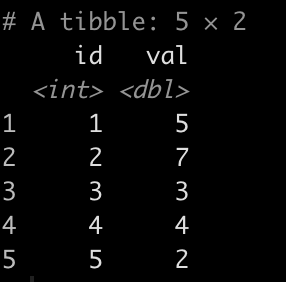
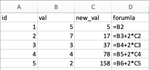
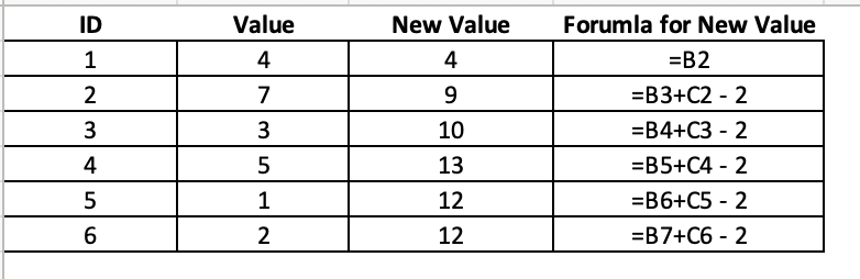
For example, in the below table we can see that we have a value for each corresponding ID. The New Value is calculated as the most recent observation of Value + lag(New Value) – 2. This is true for all observations except the first observation, which simply takes Value of the first ID observation. So, in ID 2, we get: New Value = 7 + 4 – 2 = 9 and in ID 3 we get: New Value = 3 + 9 – 2 = 10.

This type of function is pretty common in excel but it can be a little tricky in R. I’ve been meaning to do a blog about this after a few questions that I’ve gotten and Aaron Pearson reminded me about it last night, so let’s try and tackle it.

Creating Data

We will create two fake data sets:

• Data set 1 will be a larger data set with multiple subjects.
• Data set 2 will only be one subject, a smaller data set for us to first get an understanding of what we are doing before trying to perform the function over multiple people.

library(tidyverse)

## simulate data
set.seed(1)
subject <- rep(LETTERS[1:3], each = 50)
day <- rep(1:50, times = 3)
value <- c(
  round(rnorm(n = 20, mean = 120, sd = 40), 2),
  round(rnorm(n = 10, mean = 150, sd = 20), 2),
  round(rnorm(n = 20, mean = 110, sd = 30), 2),
  round(rnorm(n = 20, mean = 120, sd = 40), 2),
  round(rnorm(n = 10, mean = 150, sd = 20), 2),
  round(rnorm(n = 20, mean = 110, sd = 30), 2),
  round(rnorm(n = 20, mean = 120, sd = 40), 2),
  round(rnorm(n = 10, mean = 150, sd = 20), 2),
  round(rnorm(n = 20, mean = 110, sd = 30), 2))

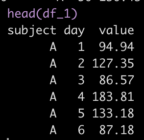
df_1 <- data.frame(subject, day, value) df_1 %>% head()

### Create a data frame of one subject for a simple example
df_2 <- df_1 %>%
  filter(subject == "A")

Exponentially Weighted Moving Average (EWMA)

We will apply an exponentially weighted moving average to the data as this type of equation requires within column aggregation.

EWMA is calculated as:

EWMA_t = lamda*x_t + (1 – lamda) * Z_t-1

Where:

• EWMA_t = the exponentially weighted moving average value at time t
• Lamda = the weighting factor
• x_t = the most recent observation
• Z_t-1 = the lag of the EWMA value

accumulate()

Within {tidyverse} we will use the accumulate() function, which allows us to create this type of within column aggregation. The function takes a few key arguments:

• First we need to pass the function the name of the column of data with our observations over time
• .y which represents the value of our most recent observation
• .f which is the function that we want to apply to our within column aggregation (in this example we will use the EWMA equation)
• .x which is going to provide us with the lagged value within the new column we are creating

Here is what it looks like in our smaller data set, df_2

df_2 <- df_2 %>%
  mutate(ewma = accumulate(value, ~ lamda * .y + (1 - lamda) * .x))

Here, we are using mutate() to create a new column called ewma. We used accumulate() and passed it the value column, which is the column of our data that has our observations and our function for calculating ewma, which follows the tilde.

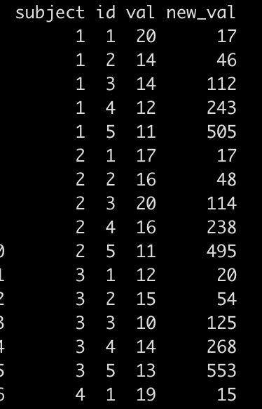
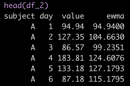
Within this function we see .y, the most recent observation and .x, the lag ewma value. By default, the first row of the new ewma column will be the first observation in the value row. Here is what the first few rows of the data look like:

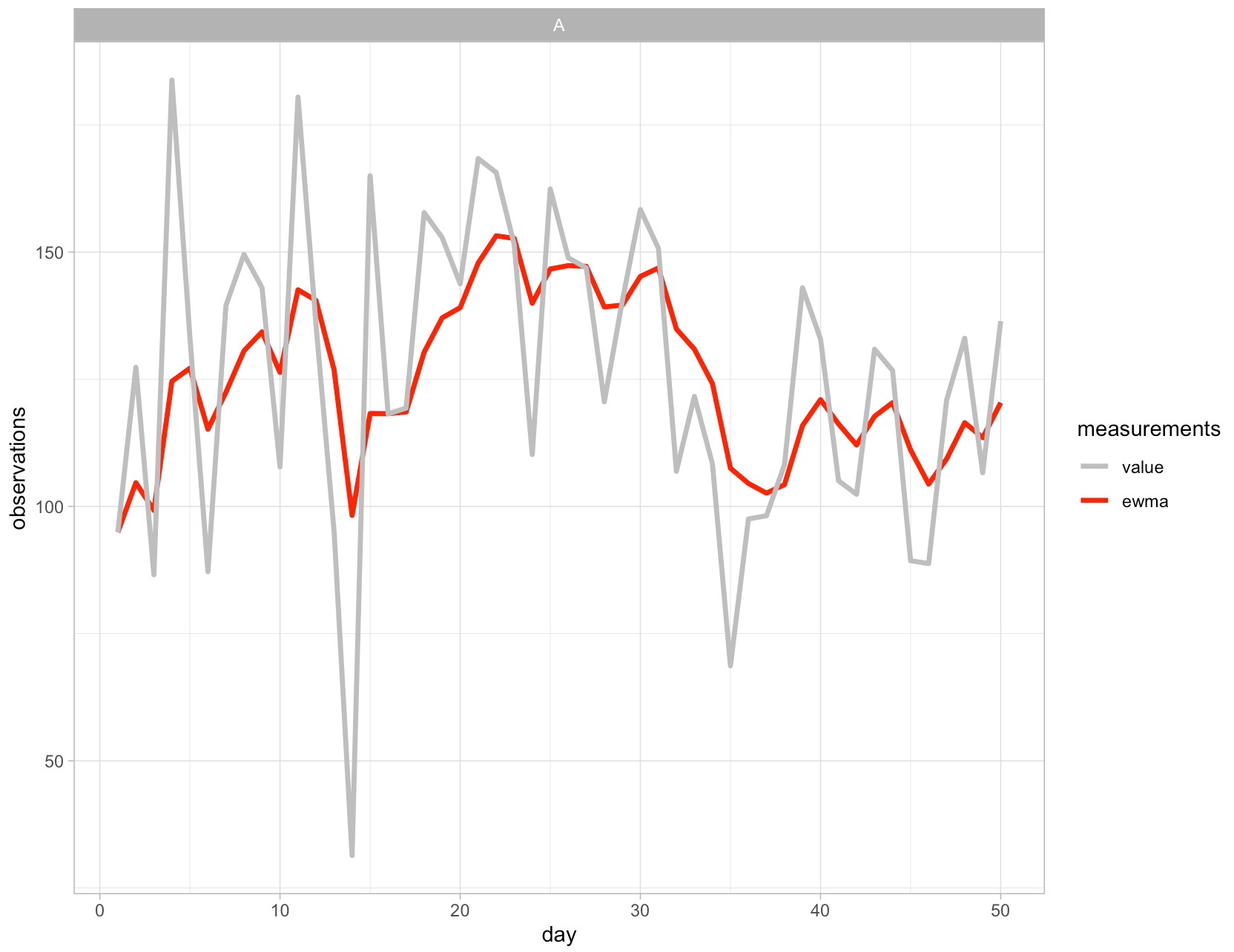
Now that new column has been created we can visualize the observed values and the EWMA values:

Applying the approach to all of the subjects

To apply this approach to all of the subjects in our data we simply need to use the group_by() function to tell R that we want to have the algorithm start over whenever it encounters a new subject ID.

df_1 <- df_1 %>%
  group_by(subject) %>%
  mutate(ewma = accumulate(value, ~ lamda * .y + (1 - lamda) * .x))

And then we can plot the outcome:

Pretty easy!

What if we want the start value to be 0 (or something else) instead of the first observation?

This is a quick fix within the accumulate() function by using the .init argument and simply passing it whatever value you want the new column to begin with. What you need to be aware of when you do this, however, is that this argument will add an additional observation to the vector of data and thus we need to remove the last row of the data set to ensure that {tidyverse} can perform the operation without giving you an error. To accomplish this, when I pass the value column to the function I add a bracket and then minus 1 of the total count, n(), of observations in that column.

df_2 %>%
  mutate(ewma = accumulate(value[-n()], ~ lamda * .y + (1 - lamda) * .x, .init = 0)) %>%
  head()

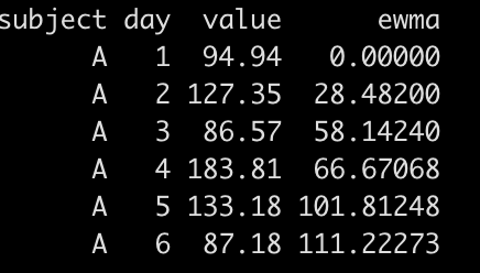
Now we see that the first value in ewma is 0 instead of 94.94, which of course changes all of the values following it since the equation is using the lagged ewma value (.x).

For the complete code, please see my GitHub Page.