The random forest algorithm is an ensemble method that fits a large number of decision trees (weak learners) and uses their combined predictions, in a wisdom of the crowds type of fashion, to make the final prediction. Although random forest can be used for classification tasks, today I want to talk about using random forest for regression problems (problems where the variable we are predicting is a continuous one). Specifically, I’m not only interested in a single prediction but I also want to get a confidence interval for the prediction.
In R, the two main packages for fitting random forests are {ranger} and {randomForest}. These packages are also the two engines available when fitting random forests in {tidymodels}. When building models in the native packages, prediction on new data can be done with the predict() function (similar to all models in R). To get an estimate of the variation in predictions, we pass the predict function the argument predict.all = TRUE, which produces a vector of all of the predictions made by each individual tree in the random forest. The problem, is that this argument is not available for predict() in {tidymodels}. Consequently, all we are left with in {tidymodels} is making a point estimate prediction (the average value of all of the trees in the forest)!!
The way we can circumvent this issue is by fitting our model in {tidymodels} using cross-validation so that we can tune the mtry and trees values. Once we have the optimum values for these hyper-parameters we will use the {randomForest} package and build a new model using those values. We will then make our predictions with this model on new data.
NOTE: I’m not 100% certain this is the best way to approach this problem inside or outside of {tidymodels}. If someone has a better solution, please drop it into the comments section or shoot me an email!
Load Packages & Data
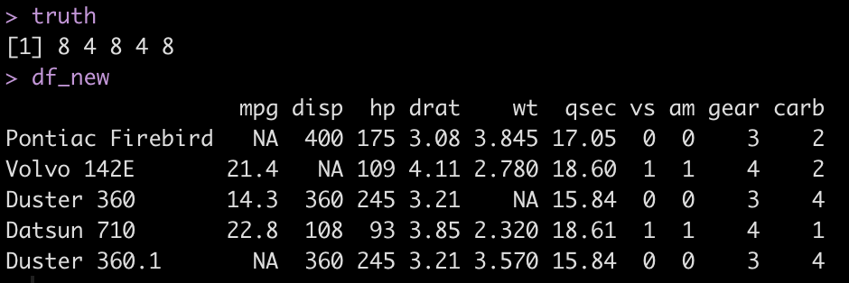
We will use the mtcars data set and try and predict the car’s mpg from the disp, hp, wt, qsec, drat, gear, and carb columns.
## Load packages
library(tidymodels)
library(tidyverse)
library(randomForest)

## load data
df <- mtcars %>%
  select(mpg, disp, hp, wt, qsec, drat, gear, carb)

head(df)
Split data into cross-validation sets
This is a small data set, so rather than spending data by splitting it into training and testing sets, I’m going to use cross-validation on all of the available data to fit the model and tune the hyper-parameters
## Split data into cross-validation sets
set.seed(5)
df_cv <- vfold_cv(df, v = 5)
Specify the model type & build a tuning grid
The model type will be a random forest regression using the randomForest engine.
The tuning grid will be a vector of values for both mtry and trees to provide the model with options to try as it tunes the hyper-parameters.
## specify the random forest regression model
rf_spec <- rand_forest(mtry = tune(), trees = tune()) %>%
  set_engine("randomForest") %>%
  set_mode("regression")

## build a tuning grid
rf_tune_grid <- grid_regular(
  mtry(range = c(1, 7)),
  trees(range = c(500, 800)),
  levels = 5
)
Create a model recipe & workflow
## Model recipe
rf_rec <- recipe(mpg ~ ., data = df)

## workflow
rf_workflow <- workflow() %>%
  add_recipe(rf_rec) %>%
  add_model(rf_spec)
Fit and tun the model
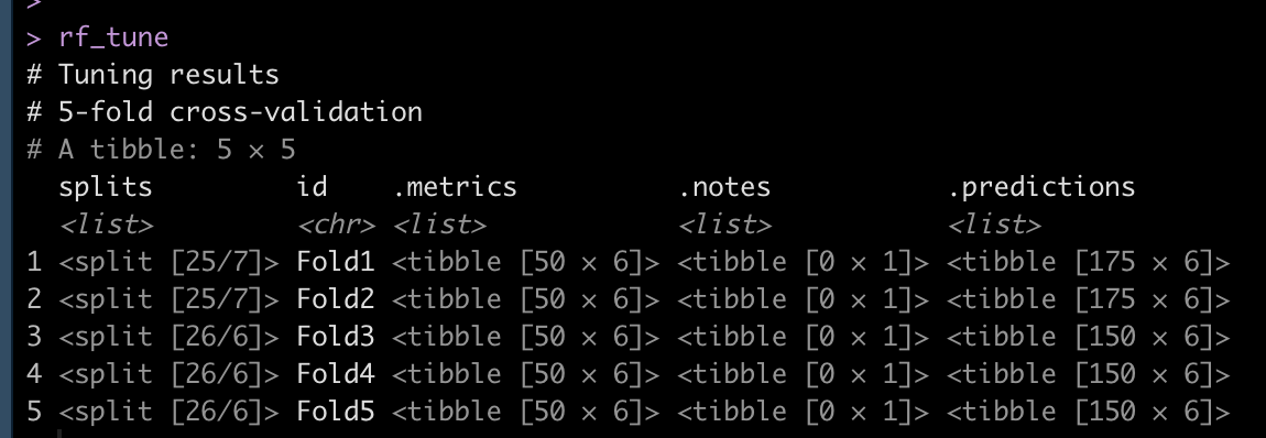
## set a control function to save the predictions from the model fit to the CV-folds
ctrl <- control_resamples(save_pred = TRUE)

## fit model
rf_tune <- tune_grid(
  rf_workflow,
  resamples = df_cv,
  grid = rf_tune_grid,
  control = ctrl
)

rf_tune
View the model performance and identify the best model
## view model metrics
collect_metrics(rf_tune)

## Which is the best model?
select_best(rf_tune, "rmse")

## Look at that models performance
collect_metrics(rf_tune) %>%
  filter(mtry == 4, trees == 725)
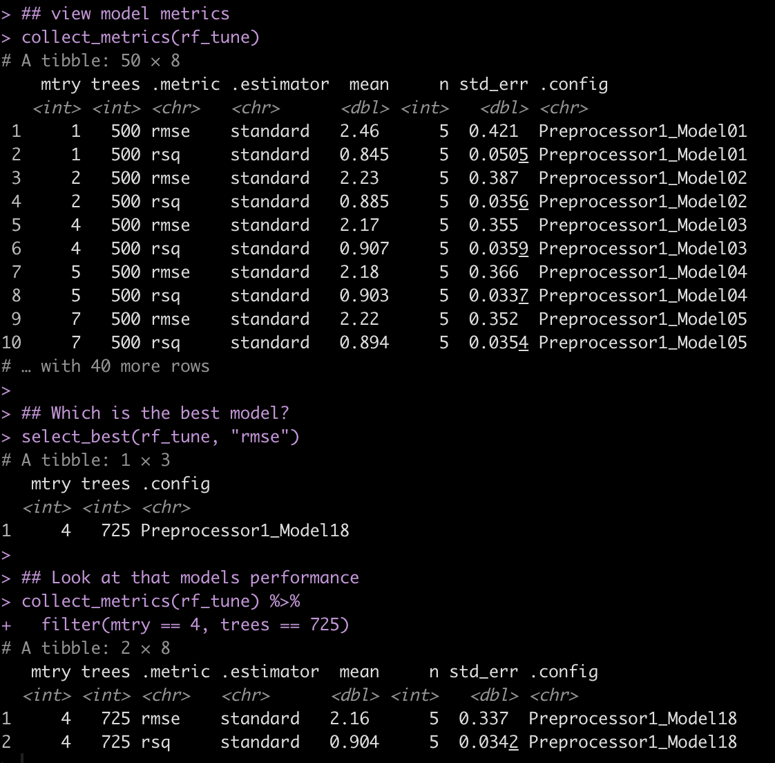
Here we see that the model with the lowest root mean squared error (rmse) has an mtry = 4 and trees = 725.
Extract the optimal mtry and trees values for minimizing rmse
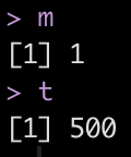
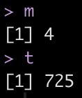
## Extract the best mtry and trees values to optimize rmse
m <- select_best(rf_tune, "rmse") %>% pull(mtry)
t <- select_best(rf_tune, "rmse") %>% pull(trees)

m
t
Re-fit the model using the optimal mtry and trees values
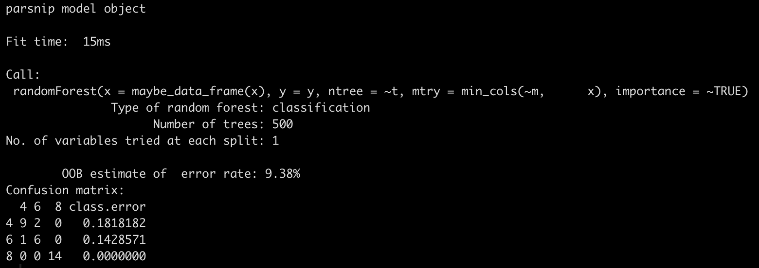
Now that we’ve identified the hyper-parameters that minimize rmse, we will re-fit the model using the {randomForest} package, so that we can get predictions for all of the trees, and specify the mtry and ntree values that were extracted from the {tidymodels} model within the function.
## Re-fit the model outside of tidymodels with the optimized values
rf_refit <- randomForest(mpg ~ ., data = df, mtry = m, ntree = t)
rf_refit
Create new data and make predictions
When making the predictions we have to make sure to pass the argument predict.all = TRUE.
## New data
set.seed(859)
row_id <- sample(1:nrow(df), size = 5, replace = TRUE)
newdat <- df[row_id, ]
newdat
## Make Predictions
pred.rf <- predict(rf_refit, newdat, predict.all = TRUE)
pred.rf
What do predictions look like?
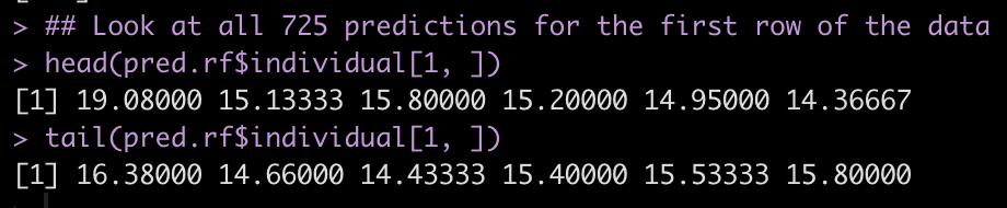
Because we requested predict all, we have the ability to see a prediction for each of the 725 trees that were fit. Below we will look at the first and last 6 predictions of the 725 individual trees for the first observation in our new data set.
## Look at all 725 predictions for the first row of the data
head(pred.rf$individual[1, ])
tail(pred.rf$individual[1, ])
What do predictions look like?
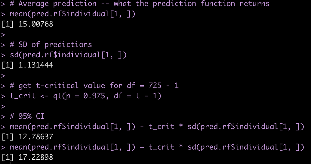
Taking the mean of the 725 predictions will produce the predicted value for the new observation, using the wisdom of the crowds. Similarly, the standard deviation of these 725 predictions will give us a sense for the variability of the weak learners. We can use this information to produce our confidence intervals. We calculate our confidence intervals as the standard deviation of predictions multiplied by the t-critical value, which we calculate from a t-distribution with the degrees of freedom equal to 725 – 1.
# Average prediction -- what the prediction function returns
mean(pred.rf$individual[1, ])

# SD of predictions
sd(pred.rf$individual[1, ])

# get t-critical value for df = 725 - 1
t_crit <- qt(p = 0.975, df = t - 1)

# 95% CI
mean(pred.rf$individual[1, ]) - t_crit * sd(pred.rf$individual[1, ])
mean(pred.rf$individual[1, ]) + t_crit * sd(pred.rf$individual[1, ])
Make a prediction with confidence intervals for all of the observations in our new data
First we will make a single point prediction (the average, wisdom of the crowds, prediction) and then we will write a for() loop to create the lower and upper 95% Confidence Intervals using the same approach as above.
## Now for all of the predictions
newdat$pred_mpg <- predict(rf_refit, newdat)

## add confidence intervals
lower <- rep(NA, nrow(newdat))
upper <- rep(NA, nrow(newdat))

for(i in 1:nrow(newdat)){
  lower[i] <- mean(pred.rf$individual[i, ]) - t_crit * sd(pred.rf$individual[i, ])
  upper[i] <- mean(pred.rf$individual[i, ]) + t_crit * sd(pred.rf$individual[i, ])
}

newdat$lwr <- lower
newdat$upr <- upper
View the new observations with their predictions and create a plot of the predictions versus the actual data
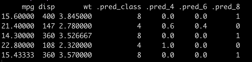
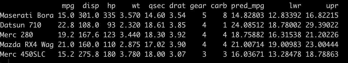
The three columns on the right show us the predicted miles per gallon and the 95% confidence interval for each of the five new observations.
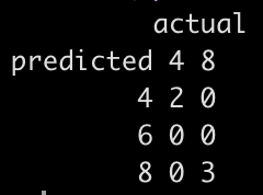
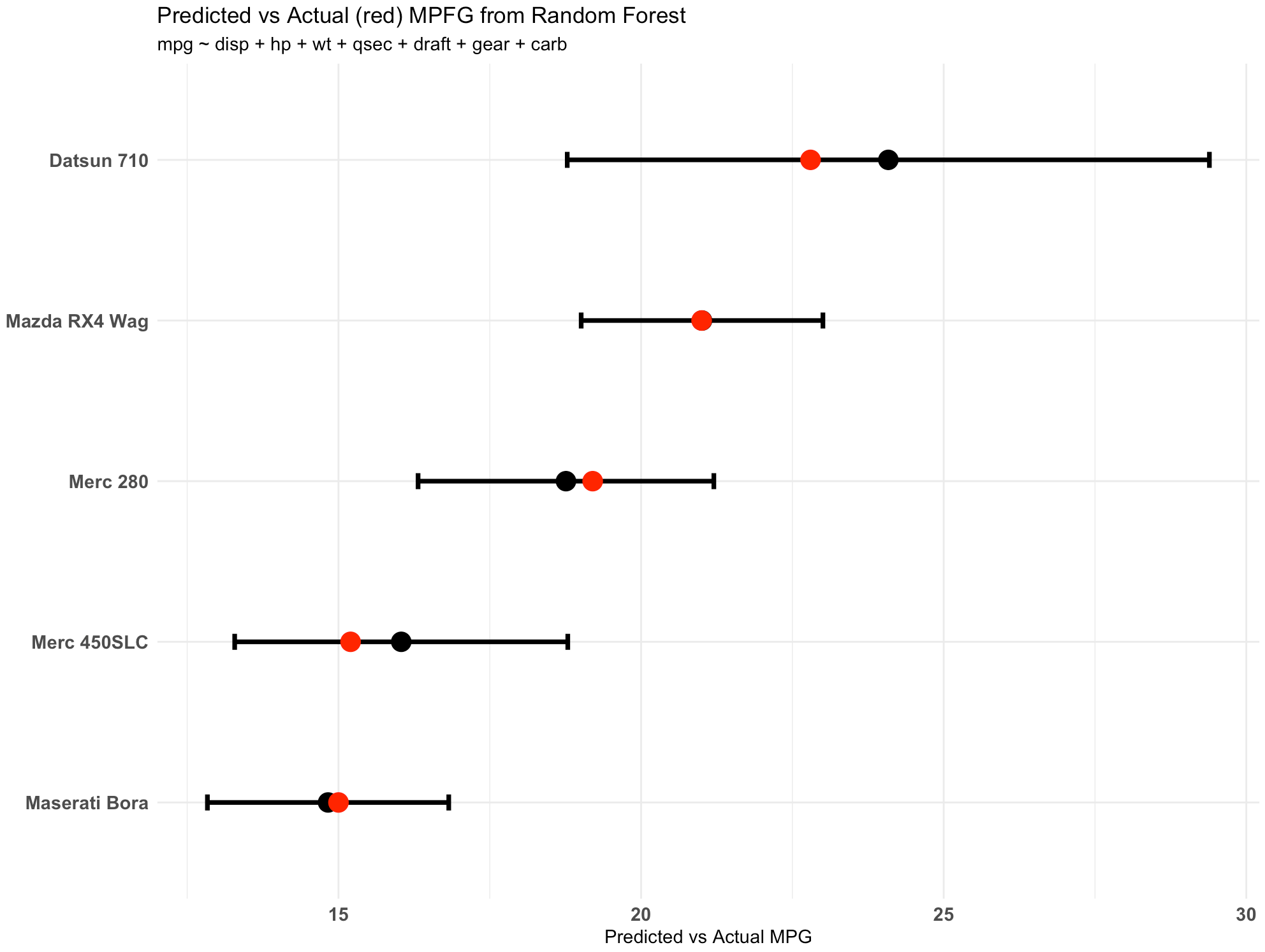
The plot shows us the point prediction and confidence interval along with the actual mpg (in red), which we can see falls within each of the ranges.
## Look at the new observations, predctions and confidence intervals and plot the data
## new data
newdat

## plot
newdat %>%
  mutate(car_type = rownames(.)) %>%
  ggplot(aes(x = pred_mpg, y = reorder(car_type, pred_mpg))) +
  geom_point(size = 5) +
  geom_errorbar(aes(xmin = lwr, xmax = upr),
                width = 0.1,
                size = 1.3) +
  geom_point(aes(x = mpg),
             size = 5,
             color = "red") +
  theme_minimal() +
  labs(x = "Predicted vs Actual MPG",
       y = NULL,
       title = "Predicted vs Actual (red) MPFG from Random Forest",
       subtitle = "mpg ~ disp + hp + wt + qsec + draft + gear + carb")
Wrapping Up
Random forests can be used for regression or classification problems. Here, we used the algorithm for regression with the goal of obtaining 95% Confidence Intervals based on the variability of predictions exhibited by all of the trees in the forest. Again, I’m not certain that this is the best way to achieve this output either inside of or outside of {tidymodels}. If anyone has other thoughts, feel free to drop them in the comments or shoot me an email.
To access all of the code for this article, please see my GITHUB page.