We’ve been working with building simulations in the past 6 articles of this series. In the last two installments we talked specifically about using simulation to explore different linear regression model assumptions. Today, we continue with linear regression and we use simulation to understand how measurement error (something we all face) influences our linear regression parameter estimates.
Here were the past 6 sections in this series:
- Part 1 discussed the basic functions for simulating and sampling data in R
- Part 2 walked us through how to perform bootstrap resampling and then simulate bivariate and multivariate distributions
- Part 3 we worked making group comparisons by simulating thousands of t-tests
- Part 4 building simulations for linear regression
- Part 5 using simulation to investigate the homoskedasticity assumption in regression
- Part 6 using simulation to investigate the multicollinearity assumption in regression
As always, complete code for this article is available on my GitHub page.
Measurement Error
Measurement error occurs when the values we have observed during data collection differ from the true values. This can sometimes be the cause of imperfect proxy measures where we are using certain measurements (perhaps tests that are easier to obtain in our population or setting) in place of the thing we actually care about. Or, it can happen because tests are imperfect and all data collection has limitations and error (which we try as hard as possible to minimize).
Measurement error can be systematic or random. It can be challenging to detect in a single sample. We will build a simulation to show how measurement error can bias our regression coefficients and perhaps hide the true relationship.
Constructing the simulation
For this simulation, we are going to use a random draw from a normal distribution for the independent variable to represent noise in the model, which will behave like measurement error. We will use a nested for() loop, as we did in Part 6 of this series, where the outer loop stores the outcomes of the regression model under each level of measurement error, which is built in the inner loop.
We begin by creating 11 levels of measurement error, ranging from 0 (no measurement error) to 1 (extreme measurement error). This values are going to serve as the standard deviation when we randomly draw from a normal distribution with a mean of 0. In this way, we are creating noise in the model.
## levels of error measurement to test
# NOTE: these values will be used as the standard deviation in our random draws
meas_error <- seq(from = 0, to = 1, by = 0.1)

# create the number of simulations and reps you want to run
n <- 1000

# true variables
intercept <- 2
beta1 <- 5
independent_var <- runif(n = n, min = -1, max = 1)

## create a final array store each of the model error levels in their own list
final_df <- array(data = NA, dim = c(n, 2, length(meas_error)))

## create a data frame to store the absolute bias at each level of measurement error
error_bias_df <- matrix(nrow = n, ncol = length(meas_error))
Next, we build our nested for() loop and simulate models under the different measurement error conditions.
## loop
for(j in 1:length(meas_error)){

  # a store vector for the absolute bias from each inner loop
  abs_bias_vect <- rep(0, times = n)

  ## storage data frame for the beta coefficient results in each inner loop simulated regression
  df_betas <- matrix(NA, nrow = n, ncol = 2)

  # simulate independent variable 1000x with measurement error
  ind_var_with_error <- independent_var + rnorm(n = n, 0, meas_error[j])

  for(i in 1:n){

    y_hat <- intercept + beta1*independent_var + rnorm(n = n, 0, 1)
    fit <- lm(y_hat ~ ind_var_with_error)

    df_betas[i, 1] <- fit$coef[1]
    df_betas[i, 2] <- fit$coef[2]

    abs_bias_vect[i] <- abs(fit$coef[2] - beta1)
  }

  ## store final results of each inner loop
  # store the model betas in a list for each level of measurement error
  final_df[, , j] <- df_betas

  # store the absolute bias
  error_bias_df[, j] <- abs_bias_vect

}
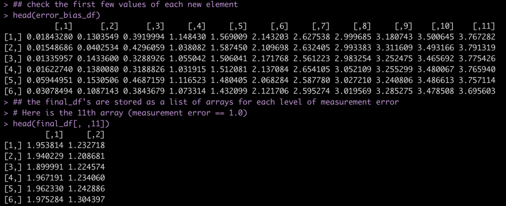
Have a look at the first few rows of each results data frame.
## check the first few values of each new element
head(error_bias_df)

## the final_df's are stored as a list of arrays for each level of measurement error
# Here is the 11th array (measurement error == 1.0)
head(final_df[, ,11])
Plotting the results
Now that we have stored the data for each level of measurement error, let’s do some plotting of the data to explore how measurement error influences our regression model.
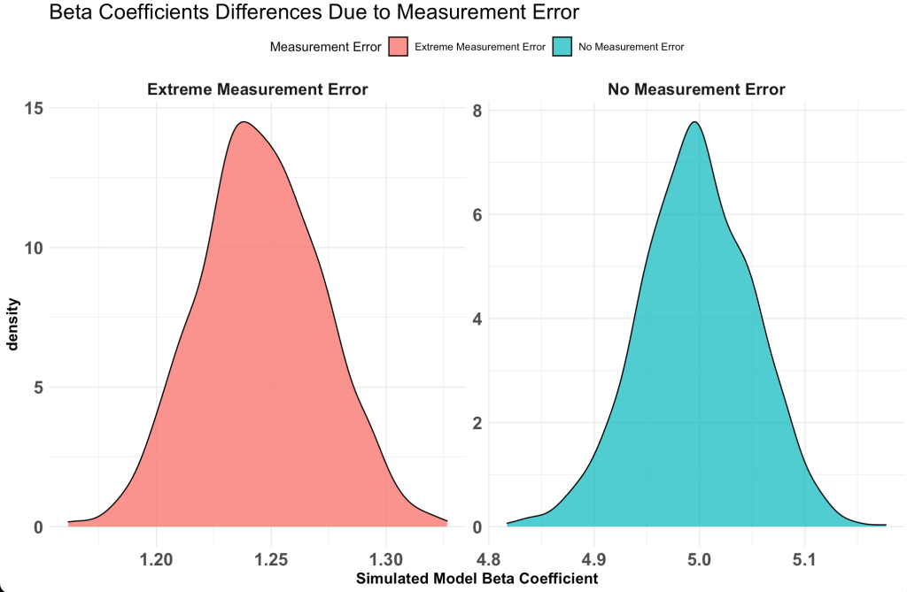
Plot the standard deviation of the beta coefficient for the model with no measurement error and the model with the most extreme measurement error.
no_error <- final_df[, ,1] %>% as.data.frame() %>% mutate(measurement_error = "No Measurement Error")

extreme_error <- final_df[, ,11] %>% as.data.frame() %>% mutate(measurement_error = "Extreme Measurement Error")

no_error %>%
  bind_rows(
    extreme_error
  ) %>%
  ggplot(aes(x = V2, fill = measurement_error)) +
  geom_density(alpha = 0.8) +
  facet_wrap(~measurement_error, scales = "free") +
  theme(strip.text = element_text(size = 14, face = "bold"),
        legend.position = "top") +
  labs(x = "Simulated Model Beta Coefficient",
       fill = "Measurement Error",
       title = "Beta Coefficients Differences Due to Measurement Error")
Notice that the value with no measurement error the beta coefficient is around 5, just as we specified the true value in our simulation. However, the model with a measurement error of 1 (shown in green) has the beta coefficient centered around 1.2, which is substantially lower than the true beta coefficient value of 5.
Plot the change in absolute bias across each level of measurement error
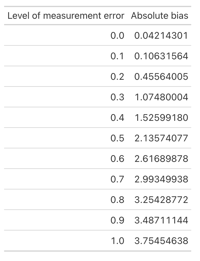
First let’s look at the average bias across each level of measurement error.
absolute_error <- error_bias_df %>%
  as.data.frame() %>%
  setNames(paste0('x', meas_error))

# On average, how much absolute bias would we expect
colMeans(absolute_error) %>%
  data.frame() %>%
  rownames_to_column() %>%
  mutate('rowname' = parse_number(rowname)) %>%
  setNames(c("Level of measurement error", 'Absolute bias')) %>%
  gt::gt()
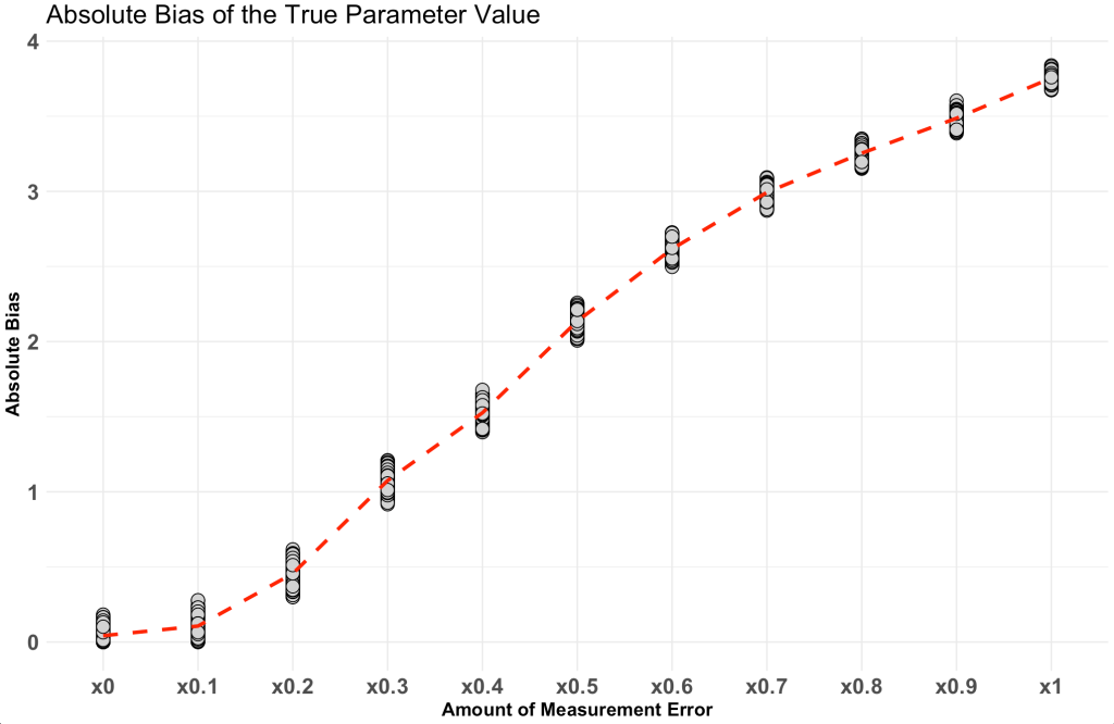
Next, make a plot of the relationship.
absolute_error %>%
  pivot_longer(cols = everything()) %>%
  ggplot(aes(x = name, y = value, group = 1)) +
  geom_point(shape = 21,
             size = 4,
             color = "black",
             fill = "light grey") +
  stat_summary(fun = mean,
               geom = "line",
               color = "red",
               size = 1.2,
               linetype = "dashed") +
  labs(x = "Amount of Measurement Error",
       y = "Absolute Bias",
       title = "Absolute Bias of the True Parameter Value")
Notice that as the amount of measurement increases so too does the absolute bias of the model coefficient.
Wrapping Up
Measurement error is something that all of us deal with in practice, whether you are conducting science in a lab or working in an applied setting. Knowing how measurement error influences regression coefficients and the tricks it can play in our beliefs to unveil true parameter values is important to keep in mind. Expressing our uncertainty around model outputs is critical to communicating what we think we know about our observations and how (un)certain we may be. This is one of the values of, in my opinion, Bayesian model building, as we can work directly with sampling from posterior distributions that provide us a way of building up distributions, which allow us to explore uncertainty and make probabilistic statements.
The complete code for this article is available on my GitHub page.


