Introduction
In {tidymodels} it is often recommended to split the data using the initial_split() function. This is useful when you are interested in a random sample from the data. As such, the initial_split() function produces a list of information that is used downstream in the model fitting and model prediction process. However, sometimes we have data that we want to fit specifically to a training set and then test on data set that we define. For example, training a model on years 2010-2015 and then testing a model on years 2016-2019.
This tutorial walks through creating your own bespoke train/test sets, fitting a model, and then making predictions, while circumventing the issues that may arise from not having the initial_split() object.
Load the AirQuality Data
library(tidyverse)
library(tidymodels)
library(datasets)

data("airquality")

airquality %>% count(Month)
Train/Test Split
We want to use `tidymodels` to build a model on months 5-7 and test the model on months 8 and 9?
Currently the initial_split() function only takes a random sample of the data.
set.seed(192)
split_rand <- initial_split(airquality ,prop = 3/4)
split_rand

train_rand <- training(split_rand)
test_rand <- testing(split_rand) train_rand %>%
  count(Month)

test_rand %>%
  count(Month)
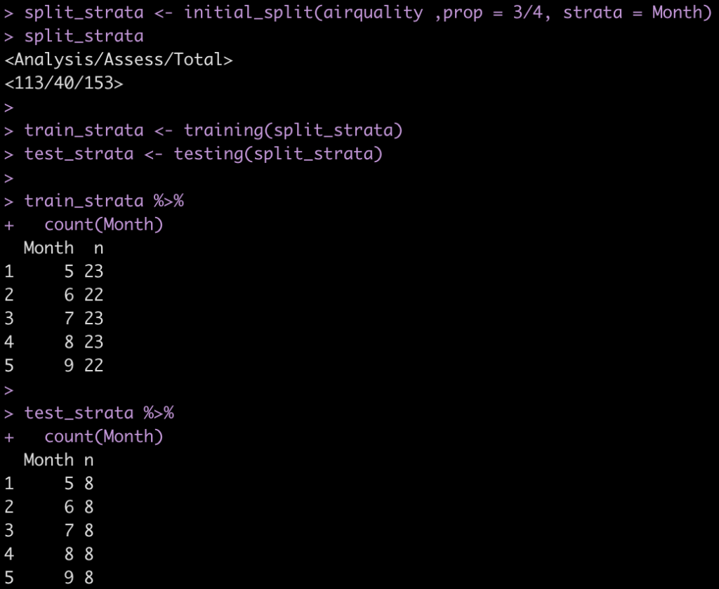
The strat argument within initial_split() only ensures that we get an even sample across our strat (in this case, Month).
split_strata <- initial_split(airquality ,prop = 3/4, strata = Month)
split_strata

train_strata <- training(split_strata)
test_strata <- testing(split_strata) train_strata %>%
  count(Month)

test_strata %>%
  count(Month)
- Create our own train/test split, unique to the conditions we are interested in specifying.
train <- airquality %>%
  filter(Month < 8)

test <- airquality %>%
  filter(Month >= 8)
- Create 5-fold cross validation for tuning our random forest model
set.seed(567)
cv_folds <- vfold_cv(data = train, v = 5)
Set up the model specification
- We will use random forest
## model specification
aq_rf <- rand_forest(mtry = tune()) %>%
  set_engine("randomForest") %>%
  set_mode("regression")
Create a model recipe
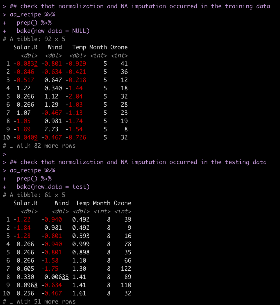
There are some NA’s in a few of the columns. We will impute those and we will also normalize the three numeric predictors in our model.
## recipe
aq_recipe <- recipe( Ozone ~ Solar.R + Wind + Temp + Month, data = train ) %>%
step_impute_median(Ozone, Solar.R) %>%
step_normalize(Solar.R, Wind, Temp)

aq_recipe

## check that normalization and NA imputation occurred in the training data
aq_recipe %>%
prep() %>%
bake(new_data = NULL)

## check that normalization and NA imputation occurred in the testing data
aq_recipe %>%
prep() %>%
bake(new_data = test)
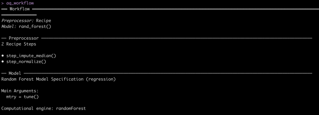
Set up workflow
- Compile all of our components above together into a single workflow.
## Workflow
aq_workflow <- workflow() %>%
add_model(aq_rf) %>%
add_recipe(aq_recipe)

aq_workflow
Tune the random forest model
- We set up one hyperparmaeter to tune, mtry, in our model specification.
## tuning grid
rf_tune_grid <- grid_regular(
  mtry(range = c(1, 4))
)

rf_tune_grid

rf_tune <- tune_grid(
  aq_workflow,
  resamples = cv_folds,
  grid = rf_tune_grid
)

rf_tune
Get the model with the optimum mtry
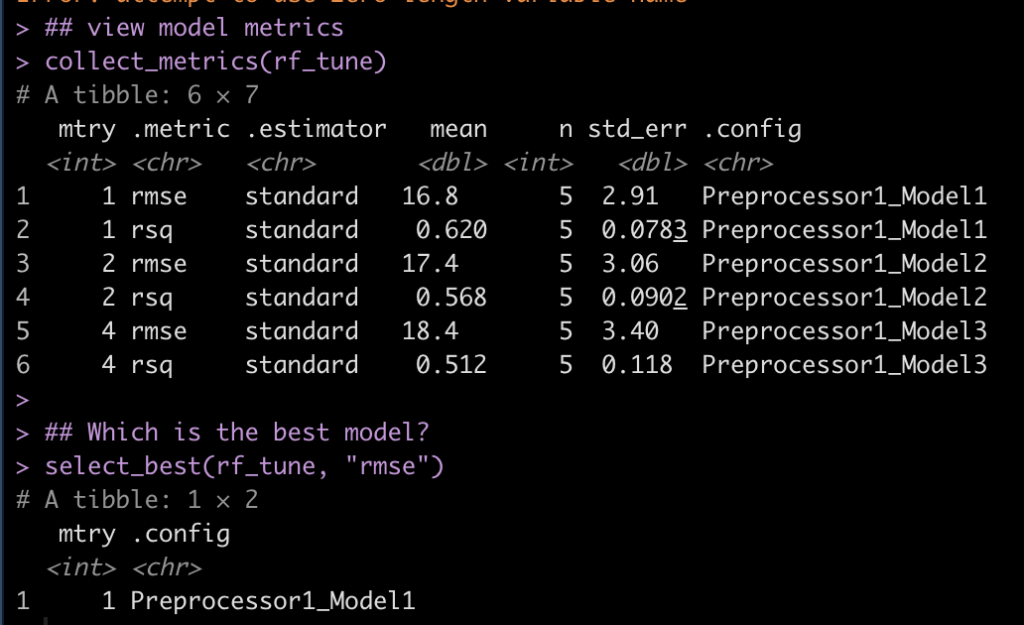
## view model metrics
collect_metrics(rf_tune)

## Which is the best model?
select_best(rf_tune, "rmse")
- Looks like an mtry = 1 was the best option as it had the lowest RMSE and highest r-squared.
Fit the final tuned model
- model specification with mtry = 1
aq_rf_tuned <- rand_forest(mtry = 1) %>%
  set_engine("randomForest") %>%
  set_mode("regression")
Tuned Workflow
- the recipe steps are the same
aq_workflow_tuned <- workflow() %>%
  add_model(aq_rf_tuned) %>%
  add_recipe(aq_recipe)

aq_workflow_tuned
Final Fit
aq_final <- aq_workflow_tuned %>%
  fit(data = train)
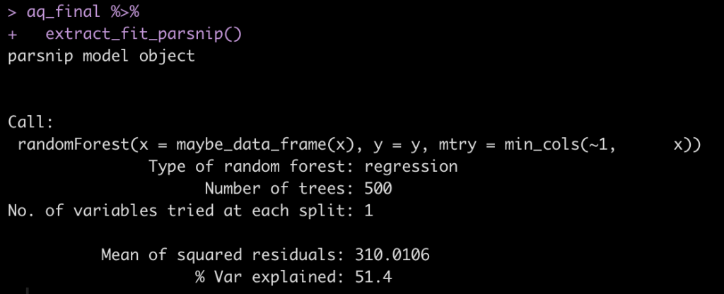
Evaluate the final model
aq_final %>%
  extract_fit_parsnip()
Predict on test set
ozone_pred_rf <- predict(
aq_final,
test
)

ozone_pred_rf
Conclusion
Pretty easy to fit a model to bespoke train/test split that doesn’t require {tidymodels} initial_split() function. Simply construct the model, do any hyperparameter tuning, fit a final model, and make predictions.
Below I’ve added the code for anyone interested in seeing this same process using linear regression, which is easier than the random forest model since there are no hyperparameters to tune.
If you’d like to have the full code in one concise place, check out my GITHUB page.
Doing the same tasks with linear regression
- This is a bit easier since it doesn’t require hyperparameter tuning.
## Model specification
aq_linear <- linear_reg() %>%
  set_engine("lm") %>%
  set_mode("regression")

## Model Recipe (same as above)
aq_recipe <- recipe( Ozone ~ Solar.R + Wind + Temp + Month, data = train ) %>%
  step_impute_median(Ozone, Solar.R) %>%
  step_normalize(Solar.R, Wind, Temp)

## Workflow
aq_wf_linear <- workflow() %>%
  add_recipe(aq_recipe) %>%
  add_model(aq_linear)

## Fit the model to the training data
lm_fit <- aq_wf_linear %>%
  fit(data = train)

## Get the model output
lm_fit %>%
  extract_fit_parsnip()

## Model output with traditional summary() function
lm_fit %>%
  extract_fit_parsnip() %>%
  .$fit %>%
  summary()

## Model output in tidy format
lm_fit %>%
  tidy()

## Make predictions on test set
ozone_pred_lm <- predict(
  lm_fit,
  test
  )

ozone_pred_lm


