We’ve worked through a number of tutorials on building simulations and in Part 4 we worked up to building simulations for linear regression. Here are the previous 4 parts:
- Part 1 discussed the basic functions for simulating and sampling data in R.
- Part 2 walked us through how to perform bootstrap resampling and then simulate bivariate and multivariate distributions.
- Part 3 we worked making group comparisons by simulating thousands of t-tests
- Part 4 building simulations for linear regression
There are a number of assumptions that underpin linear regression models. Simulation can be a useful way of exploring these assumptions and understanding how violating these assumptions can lead to bias, large variance in the regression coefficients, and/or poor predictions.
Some typical assumptions include:
- Homoskedasticity
- Multicollinearity of independent variables
- Measurement Error
- Serial correlation
Today, we will explore the assumption of homoskedasticity.
As always, all code is freely available in the Github repository.
Creating the baseline simulation
Before exploring how violations of the homoskedasticity assumption influence a regression model, we need a baseline model to compare it against. So, we will begin by simulating a simple linear regression with 1 predictor. Our model will look like this:
y = 2 + 5*x + e
Where e will be random error from a normal distribution with a mean of 0 and standard deviation of 1.
The code below should look familiar as we’ve been building up simulations like this in the previous 4 tutorials. We specify the intercept to be 2 and the slope to be 5. The independent variable, x, is drawn from a uniform distribution between -1 and 1. With each of the 500 iterations of the for() loop we store the simulated intercept, slope, and their corresponding standard errors, which we calculate using the variance-covariance matrix (which we discussed in the previous tutorial). Finally, we also store the residual standard error (RSE) of each of the simulated models.
library(tidymodels)
library(patchwork)
## set seed for reproducibility
set.seed(58968)
## create a data frame to store intercept values, slope values, their standard errors, and the model residual standard error, for each simulation
sim_params <- data.frame(intercept = NA,
slope = NA,
intercept_se = NA,
slope_se = NA,
model_rse = NA)
# true intercept value
intercept <- 2
# true slope value
slope <- 5
## Number of simulations to run
n <- 500
# random draw from a uniform distribution to simulate the independent variable
X <- runif(n = n, min = -1, max = 1)
## loop for regression model
for(i in 1:n){
# create dependent variable, Y
Y <- intercept + slope*X + rnorm(n = n, mean = 0, sd = 1)
# build model
model <- lm(Y ~ X)
## store predictions
fitted_vals <- model$fitted.values
## store residuals
# output_df[i, 2] <- model$residuals
# variance-covariance matrix for the model
vcv <- vcov(model)
# estimates for the intercept
sim_params[i, 1] <- model$coef[1]
# estimates for the slope
sim_params[i, 2] <- model$coef[2]
# SE for the intercept
sim_params[i, 3] <- sqrt(diag(vcv)[1])
# SE for the slope
sim_params[i, 4] <- sqrt(diag(vcv)[2])
# model RSE
sim_params[i, 5] <- summary(model)$sigma
}
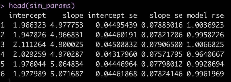
head(sim_params)
Now we summarize the data to see if we have values close to the specified model parameters.
sim_params %>%
  summarize(across(.cols = everything(),
                   ~mean(.x)))
The average intercept and slope of the 500 simulated models are pretty much identical to the specified intercept and slope of 2 and 5, respectively.
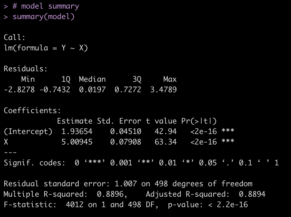
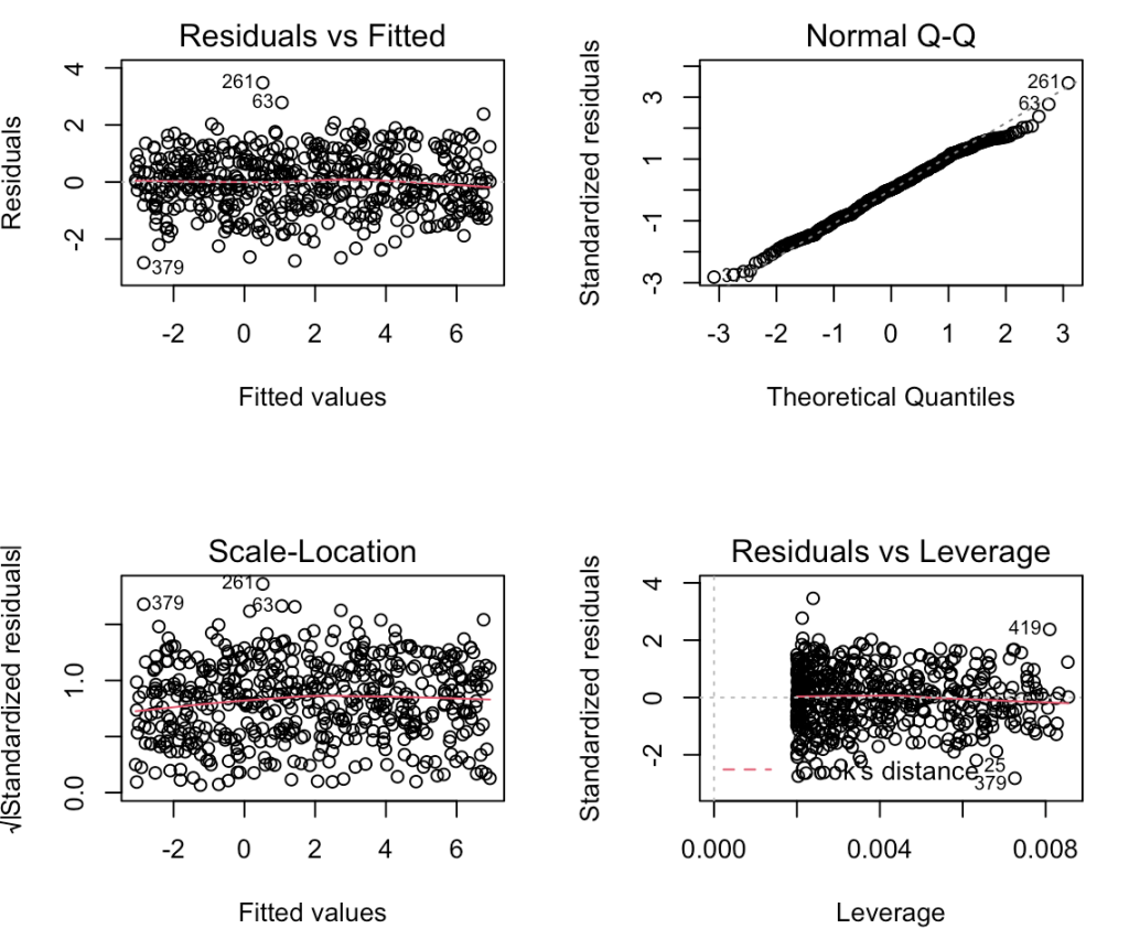
The final model of the 500 iterations is also stored from our for loop and we can look directly at it and create plots of the model fit.
# model summary
summary(model)

# model fit plots
par(mfrow = c(2,2))
plot(model)
We can also create a function that lets us evaluate how often the 95% confidence interval of our simulated beta coefficients cover the true beta coefficients that we specified for the simulation. From there, we can get a coverage probability and a 95% probability coverage interval.
### Create a coverage probability function
coverage_interval95 <- function(beta_coef, se_beta_coef, true_beta_val, model_df){
level95 <- 1 - (1 - 0.95) / 2
# lower 95
lower95 <- beta_coef - qt(level95, df = model_df)*se_beta_coef
# upper 95
upper95 <- beta_coef + qt(level95, df = model_df)*se_beta_coef
# what rate did we cover the true value (hits and misses)
hits <- ifelse(true_beta_val >= lower95 & true_beta_val <= upper95, 1, 0)
prob_cover <- mean(hits)
# create the probability coverage intervals
low_coverage_interval <- prob_cover - 1.96 * sqrt((prob_cover * (1 - prob_cover)) / length(beta_coef))
upper_coverage_interval <- prob_cover + 1.96 * sqrt((prob_cover * (1 - prob_cover)) / length(beta_coef))
# results in a list
return(list('Probability of Covering the True Value' = prob_cover,
'95% Prob ability Coverage Intervals' = c(low_coverage_interval, upper_coverage_interval)))
}
Let’s apply the function to the intercept.
coverage_interval95(beta_coef = sim_params$intercept,
                    se_beta_coef = sim_params$intercept_se,
                    true_beta = intercept,
                    model_df = model$df.residual)
Now apply the function to the slope.
coverage_interval95(beta_coef = sim_params$slope,
                    se_beta_coef = sim_params$slope_se,
                    true_beta = slope,
                    model_df = model$df.residual)
In both cases we are covering the true betas around 95% of the time, with relatively small intervals.
Homoskedasticity
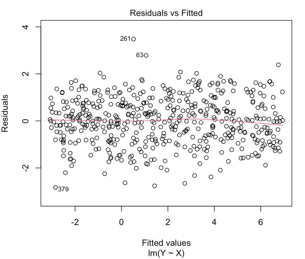
Linear models make an assumption that the variance of the residuals remain constant across the predicted values (homoskedastic). We can see what this looks like by plotting the fitted values relative to the residuals, which was the first plot in the model check plots we created for the 500th simulation above. We can see that the residuals exhibit relatively the same amount of variance across the fitted values.
plot(model, which = 1)
Let’s simulate a model with heteroskedastic residuals and see what it looks like. We will keep the same intercept and slope parameters as above. The only thing will we do is add an exponential parameter to the error term of the model to create a heteroskedastic outcome in the residuals.
## parameter for heteroskedasticity
heteroskedasticity_param <- 2

## set seed for reproducibility
set.seed(22)

## data frame for results
heteroskedastic_sim_params <- data.frame(intercept = NA,
                      slope = NA,
                      intercept_se = NA,
                      slope_se = NA,
                      model_rse = NA)

## for loop
for(i in 1:n ){

  # the error variance of Y is a function of X plus some random noise
  Y <- intercept + slope*X + rnorm(n = n, mean = 0, sd = exp(X*heteroskedasticity_param))

  # model
  heteroskedastic_model <- lm(Y ~ X)


  # variance-covariance matrix
  vcv <- vcov(heteroskedastic_model)

  # estimates for the intercept
  heteroskedastic_sim_params[i, 1] <- heteroskedastic_model$coef[1]

  # estimates for the slope
  heteroskedastic_sim_params[i, 2] <- heteroskedastic_model$coef[2]

  # SE for the intercept
  heteroskedastic_sim_params[i, 3] <- sqrt(diag(vcv)[1])

  # SE for the slope
  heteroskedastic_sim_params[i, 4] <- sqrt(diag(vcv)[2])

  # model RSE
  heteroskedastic_sim_params[i, 5] <- summary(heteroskedastic_model)$sigma

}

head(heteroskedastic_sim_params)


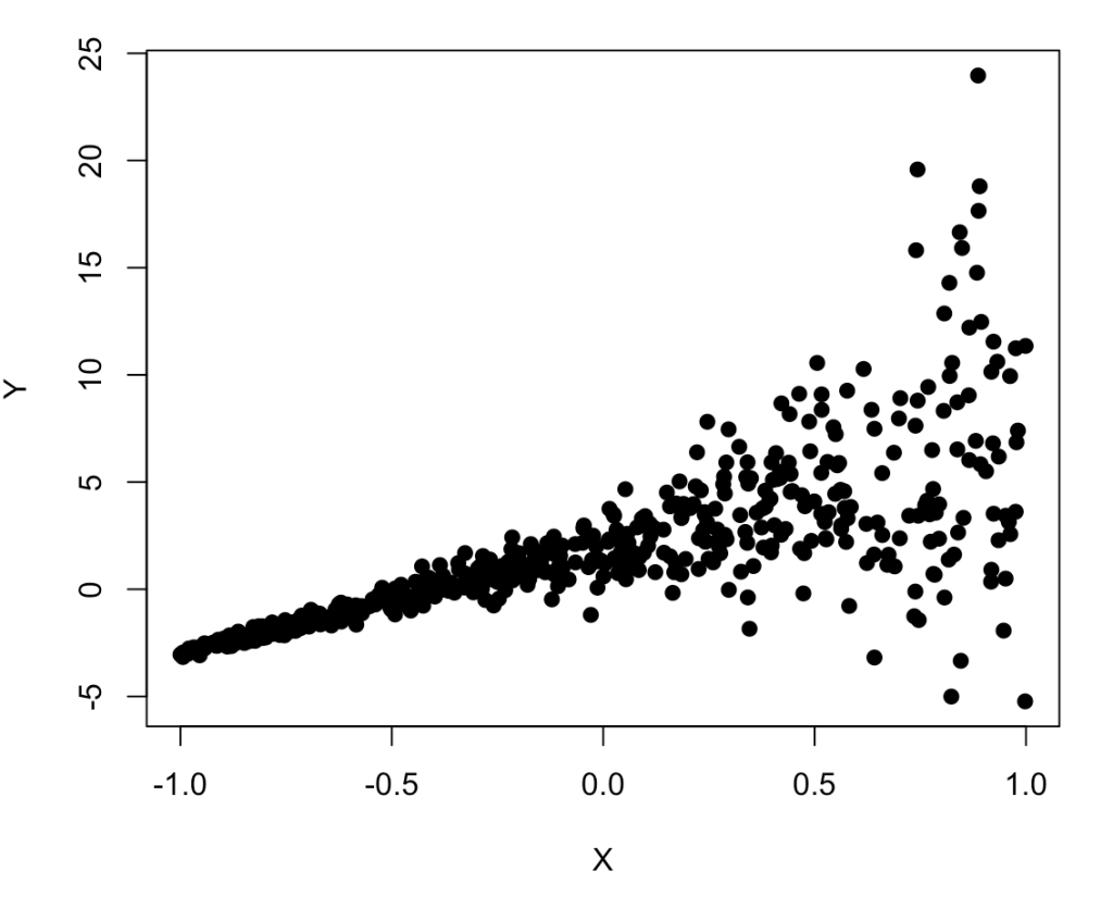
plot(X, Y, pch = 19)
The relationship between X and Y certainly looks weird given how it starts very tightly on the left side and then fans out on the right side.
Let’s take the average across all 500 simulations for each coefficient and their corresponding standard errors.
heteroskedastic_sim_params %>%
  summarize(across(.cols = everything(),
                   ~mean(.x)))
The coefficients of 2.0 for the intercept and 5 for the slope are exactly what we set them as for the simulation. However, notice how much larger the standard errors are for the intercept and slope compared to the original model above. Additionally, notice that the model residual standard error has increased substantially compared to the previous model.
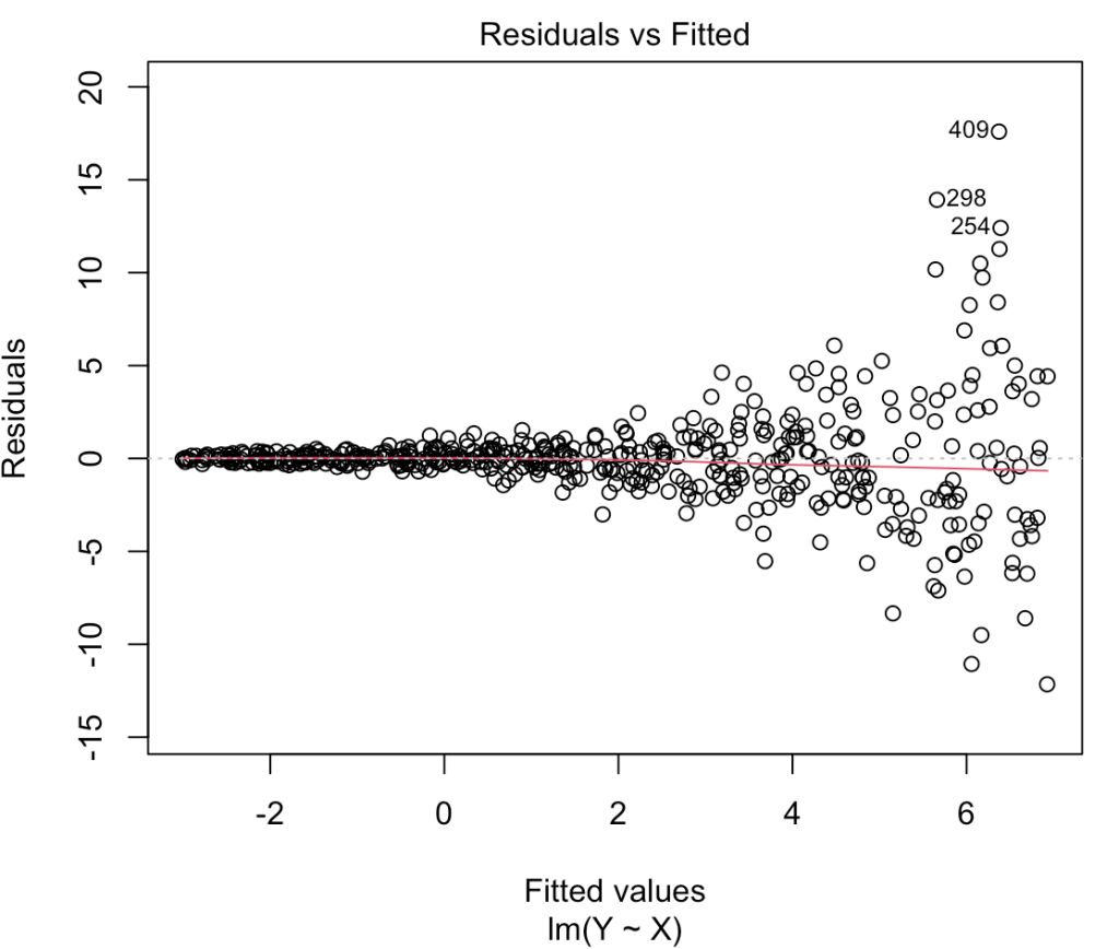
Let’s get the 500th model again and check out the fitted vs residual plot.
# fitted vs residuals
plot(heteroskedastic_model, which = 1)
That looks like a large amount of heteroskedasticity as the residual variance is no longer homogenous across the range of fitted values. Notice the large fanning out towards the right side of the plot. As the predictions get larger so two does the variability in residuals, which we noticed when we plotted Y and X above.
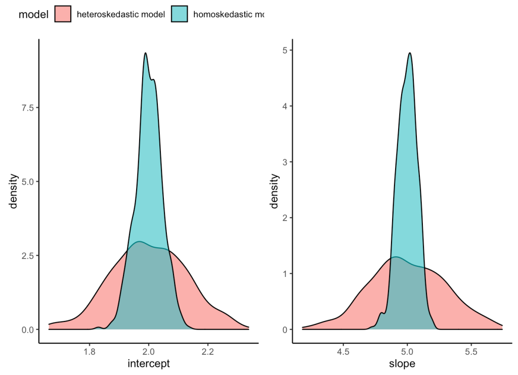
What we’ve learned is that the estimate of intercept and slope is unbiased for both the heteroskedastic and homoskedastic models, as they both are centered on the parameters that we specified for the simulation (intercept = 2, slope = 5). However, the heteroskedastic model creates greater variance in our coefficients. We can visualize how much uncertainty there is under the heteroskedastic model relative to the homoskedastic model by visualizing the density of the coefficient estimates from our two model simulations.
plt_intercept <- sim_params %>%
  mutate(model = 'homoskedastic model') %>%
  bind_rows(
    heteroskedastic_sim_params %>%
      mutate(model = 'heteroskedastic model')
  ) %>%
  ggplot(aes(x = intercept, fill = model)) +
  geom_density(alpha = 0.6) +
  theme_classic() +
  theme(legend.position = "top")

plt_slope <- sim_params %>%
  mutate(model = 'homoskedastic model') %>%
  bind_rows(
    heteroskedastic_sim_params %>%
      mutate(model = 'heteroskedastic model')
  ) %>%
  ggplot(aes(x = slope, fill = model)) +
  geom_density(alpha = 0.6) +
  theme_classic() +
  theme(legend.position = "none")

plt_intercept | plt_slope
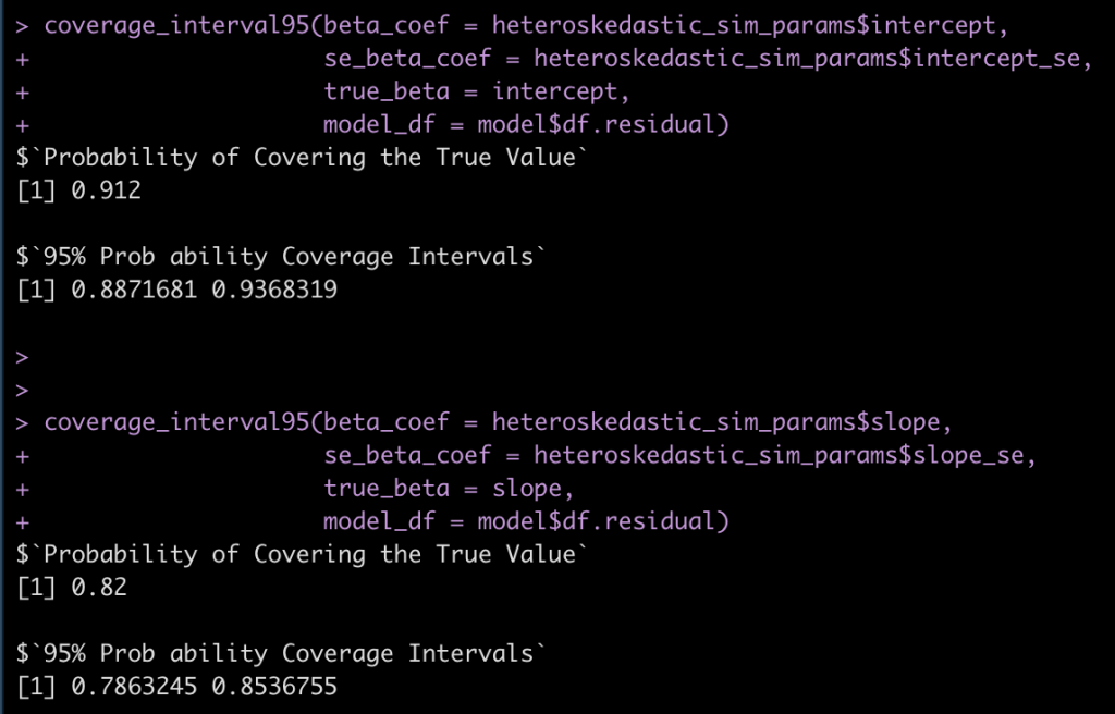
Finally, let’s see how often the 95% coverage interval is covering the true intercept and slope in the heteroskedastic model.
coverage_interval95(beta_coef = heteroskedastic_sim_params$intercept,
                    se_beta_coef = heteroskedastic_sim_params$intercept_se,
                    true_beta = intercept,
                    model_df = model$df.residual)


coverage_interval95(beta_coef = heteroskedastic_sim_params$slope,
                    se_beta_coef = heteroskedastic_sim_params$slope_se,
                    true_beta = slope,
                    model_df = model$df.residual)
Notice that we are no longer covering the true model values at the 95% level.
Wrapping Up
Simulations can be useful for evaluating model assumptions and seeing how a model may be have under different circumstances. In this tutorial we saw that a model suffering from severe heteroskedasticity is still able to return the true values for the intercept and slope. However, the variance around those values is large, meaning that we have a lot of uncertainty about what those true parameters actually are. In upcoming tutorials we will explore other linear regression assumptions. If this is a topic you enjoy, a book that I recommend (which heavily influenced today’s tutorial) is Monte Carlo Simulation and Resampling Methods for Social Sciences by Carsey & Harden.
As always, all code is freely available in the Github repository.

