To review where we are at so far:

• Part 1 discussed the basic functions for simulating and sampling data in R.
• Part 2 walked us through how to perform bootstrap resampling and then simulate bivariate and multivariate distributions.

In Part 3, we are ready to put this info to use and start to simulate data and construct models. To start things off, this tutorial will focus on simulating data for comparison of group means — a t-test.

As always, all code is freely available in the Github repository.

Simulating Two Groups for Comparison

We begin by simulating two groups using the rnorm() function to make a random draw from a normal distribution. Group 1 will have a mean of 50 and a standard deviation of 10 while Group 2 will have a mean of 60 with a standard deviation of 6.25. Both groups have a sample size of 10 (so this is a small study!).

In addition to simulating the data, we will store summary statistics for each group so that we can use them later.

set.seed(1759)
grp1 <- rnorm(n = 10,
              mean = 50,
              sd = 10)

grp2 <- rnorm(n = 10,
              mean = 60,
              sd = 6.25)

## get the summary statistics for both groups
# sample size
n_grp1 <- length(grp1)
n_grp2 <- length(grp2)

# means
mu_grp1 <- mean(grp1)
mu_grp2 <- mean(grp2)

# variances
var_grp1 <- var(grp1)
var_grp2 <- var(grp2)

# standard deviation
sd_grp1 <- sd(grp1)
sd_grp2 <- sd(grp2)

Next, we calculate the t-statistic, which is the difference between the two groups means divided by the pooled standard deviation of the two groups.

## pooled SD
sd_pool <- sqrt(((n_grp1 - 1) * var_grp1 + (n_grp2 - 1) * var_grp2) / (n_grp1 + n_grp2 - 2))
sd_pool

## Compute t-statistic
t_stat <- (mu_grp1 - mu_grp2) / (sd_pool * sqrt(1/n_grp1 + 1/n_grp2))
t_stat

We can use this t-statistic to determine if the difference is significant or not at a desired alpha level, say p < 0.05, by using a t-distribution (the qt() function, which we were introduced to in Part 1 of this series). We then check our work against R’s build in t.test() function.

alpha <- 0.05
df <- n_grp1 + n_grp2 - 2 if(abs(t_stat) > qt(1 - alpha / 2, df, lower.tail = TRUE)){
  "significant difference"} else {"not a significant difference"} 

# Get p-value
p_value <- 2*pt(abs(t_stat), df, lower=FALSE)
p_value

# check work
t.test(grp1, grp2)

The group difference is barely significant at the p < 0.05 level. We calculated the t-statistic by hand and got the exact same value as that which was produced by the t.test() function.

To make this approach more streamlined, let’s create our own t-test function so that all we need to do in the future is pass it a vector of values representing each group’s data and get returned the t-statistic.

 

## t-test function
t_stat_func <- function(x, y){
  n_grp1 <- length(x)
  n_grp2 <- length(y)
  sd_pool <- sqrt(((n_grp1 - 1) * sd(x)^2 + (n_grp2 - 1) * sd(y)^2) / (n_grp1 + n_grp2 - 2))
  t_stat <- (mean(x) - mean(y)) / (sd_pool * sqrt(1/n_grp1 + 1/n_grp2))
  return(t_stat)
}

## try out the function
t_stat_func(x = grp1, y = grp2)

We only have 10 observations in each of our groups. With such a small sample size, it may be challenging to really know if the difference we observed is real or just some sort of chance/luck occurrence (we will explore sample size issues via simulation in a later blog post). What we can do is use the function we just created and build simulated distributions using the data generating process (mean and SD) of each group to run a Monte Carlo simulations and explore how often we might reject or accept the null hypothesis at an alpha level of p < 0.05.

# Let's set alpha to 0.05
alpha <- 0.05

# We will run 10,000 simulations
N_sims <- 1e4

# create an empty vector for storing t-statistics and p-valies
t_stat <- rep(NA, N_sims)
p_values <- rep(NA, N_sims)

for(i in 1:N_sims){
  
  # simulate population 1
  grp1_sim <- rnorm(n = n_grp1, mean = mu_grp1, sd = sd_grp1)
  
  # simulate group 2
  grp2_sim <- rnorm(n = n_grp2, mean = mu_grp2, sd = sd_grp2)
  
  # compute the t-statistic with our function
  t_stat[i] <- t_stat_func(grp1_sim, grp2_sim)

  # get degrees of freedom for calculating the p-value
  df <- n_grp1 + n_grp2 - 2
  
  # obtain the p-value
  p_value[i] <- 2*pt(abs(t_stat[i]), df, lower=FALSE)
}

par(mfrow = c(1, 2))
hist(abs(t_stat),
     main = "T-Statistic Distribution")
abline(v = mean(abs(t_stat)),
       col = "red",
       lwd = 3,
       lty = 2)
hist(p_value,
     main = "p-value Distribution")
abline(v = 0.05,
       col = "red",
       lwd = 3,
       lty = 2)

# What percentage of times did we reject the null?
mean(p_value < 0.05)

You will get slightly different results, since I didn’t set a seed, but you will find that we end up rejecting the null about 52-53% of the time, meaning we probably wouldn’t want to be too confident about our “statistically significant” finding.

We could have saved a lot of lines of code and instead used the replicate() function and run 10,000 simulations of the t-test between the two groups (additionally, replicate() will run faster than the for() loop).

 

t_test <- function(){
  grp1 <- rnorm(n = n_grp1, mean = mu_grp1, sd = sd_grp1)
  grp2 <- rnorm(n = n_grp2, mean = mu_grp2, sd = sd_grp2)
  t_stat_func(grp1, grp2)
}


# Instead of a for loop, we will use the replicate() function to run this 10,000 times
t_stat_vector <- replicate(n = 10000,
                           t_test())

head(t_stat_vector)
hist(abs(t_stat_vector),
     main = "T-Test Simulation using replicate()",
     xlab = "T-Statistic")

Simulating Data from Studies

Why just create fake data and play around when we can use a similar approach to simulating data to help us further explore data contained in studies we read?! Most studies do not provide full data sets but do provide necessary summary statistics (e.g., sample size, mean, standard deviation, standard errors, confidence intervals, etc.), allowing us to use the data generating processes to simulate the study.

I was reading a 2010 paper from Saenz et al., Knee isokinetic test-retest: A multicenter knee isokinetic test-retest study of a fatigue protocol (Eur J Phys Rehabil Med), where they authors were conducing a series of test-retest protocols using a biodex. The tables in the paper lay out the information required to simulate the study. For example, in Table 1, the authors’ provide the mean, median, and standard deviation for all of the extension tests that were performed. I’ll use the data provided for the test, WRepMax.

## Saenz (2010) - Knee isokinetic test-retest - simulation
## Table 1: Extension
# We will simulate the test scores provided for WrepMax

# number of subjects
N <- 90

## Get the mean and SD for the test and retest from Table 1 for WrepMax
test1_mu <- 99.3
test1_sd <- 18.34
test2_mu <- 104.44
test2_sd <- 24.90

Next, we calculate the mean difference between test 1 and test 2 and grab the standard deviation for the test, provided in Table 3 of the paper.

## Get the difference and standard deviation of the difference between test 1 and 2 from Table 3 (row 1)
diff <- test1_mu - test2_mu
sd_diff <- 17.37

First, we simulate Test 1 using the above parameters (sample size, mean, and standard deviation).

## Simulate the first test using the summary statistics from Table 1
set.seed(925)
w_rep_max_1 <- rnorm(n = N, mean = test1_mu, sd = test1_sd)

Next, we simulate Test 2. However, we have to remember consider that, because we are trying to simulate the performance of the 90 participant in the study, Test 2 has a relationship to the performance of Test 1 because the authors’ are analyzing the difference in performance between the two tests. Therefore, to create Test 2 we will use our simulation of Test 1 for each participant and include some random error, which is specific to the mean and standard deviation of the difference between Test 1 and Test 2 reported in the study.

## Simulate test 2 by taking test 1 and applying the observed difference between tests (Table 3) 
set.seed(479)
w_rep_max_2 <- w_rep_max_1 + rnorm(n = N, mean = abs(diff), sd = sd_diff)

Now that we have Test 1 and Test 2 simulated for each participant, we can calculate the summary statistics and see how well they compare to the observed data reported in the study.

## Get the mean and SD of the simulated test1 and test 2
test1_mu_sim <- mean(w_rep_max_1) 
test1_sd_sim <- sd(w_rep_max_1)

test2_mu_sim <- mean(w_rep_max_2)
test2_sd_sim <- sd(w_rep_max_2)

test1_mu_sim
test1_sd_sim

test2_mu_sim
test2_sd_sim

## Get the mean and SD of the difference between simulations
diff_mu_sim <- mean(w_rep_max_1 - w_rep_max_2)
diff_sd_sim <- sd(w_rep_max_1 - w_rep_max_2)

diff_mu_sim
diff_sd_sim

The results are nearly identical to those presented in the study (see the link, as the study is free). Now that we have a simulated data set of all of the participants we can do other things with the data, such as plot it, conduct additional reliability metrics that weren’t performed in the study, recreate the analysis in the study to get a better understanding of the analysis that was performed, or perhaps try and model the data in different ways to explore its properties and generate new ideas for future research.

For example, let’s run a paired t-test on the simulated data, as the author’s did and look at the results in comparison to simulating this study 1000 times. We re-write our t_test() function from above to re-simulate the data in the study and then conduct a paired t-test, storing the t-statistic so that we can investigate how often we would reject the null hypothesis.

## Run a paired t-test
t.test(w_rep_max_1, w_rep_max_2, paired = TRUE)

## create a function for the paired t-test and extract the t-statistic
t_test_retest <- function(){
  w_rep_max_1 <- rnorm(n = N, mean = test1_mu, sd = test1_sd)
  w_rep_max_2 <- w_rep_max_1 + rnorm(n = N, mean = abs(diff), sd = sd_diff)
  t.test(w_rep_max_1, w_rep_max_2, paired = TRUE)$statistic
}

# Instead of a for loop, we will use the replicate() function to run this 10,000 times
t_stat_test_retest <- replicate(n = 10000,
                           t_test_retest())

hist(t_stat_test_retest)
mean(t_stat_test_retest)

# turn the t-statistics into p-values
p <- 2*pt(abs(t_stat_test_retest), df = 90 - 2, lower=FALSE)

# histogram of p-values
hist(p,
     main = "p-values of all simulated data\nreject the null ~79% of the time")

# what percentage of times did we reject the null at the p < 0.05 level?
mean(p < 0.05)

We reject the result approximately 79% of the time at the alpha level of p < 0.05.

Wrapping Up

This tutorial worked through using simulation to understand the difference in group means, as we would commonly do with a t-test. Next, we progress on to simulation linear regression models.

As always, all code is freely available in the Github repository.

In Part 1 of this series we covered some of the basic functions that we will need to perform resampling and simulations in R.

In Part 2 we will now move to building bootstrap resamples and simulating distributions for both bivariate and multivariate relationships. Some stuff we will cover:

• Coding bootstrap resampling by hand for both a single variable (mean) and regression coefficients.
• Using the boot() function from the boot package to perform bootstrapping for both a single variable and regression coefficients.
• Creating a simulation where two variables are in some way dependent on each other (correlate).
• Creating a simulation where multiple variables are correlated with each other.
• Finally, to understand what is going on with these simulated distributions we will also work through code that shows us the relationship between variables using both covariance and correlation matrices.

As always, all code is freely available in the Github repository.

Resampling

The resampling approach we will use here is bootstrapping. The general concept of bootstrapping is as follows:

• Draw multiple random samples from observed data with replacement.
• Draws must be independent and each observation must have an equal chance of being selected.
• The bootstrap sample should be the same size as the observed data in order to use as much information from the sample as possible.
• Calculate the mean resampled data and store it.
• Repeat this process thousands of times and summarize the mean of resampled means and the standard deviation of resampled means to obtain summary statistics of your bootstrapped resamples.

Write the bootstrap resampling by hand

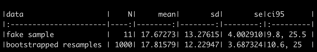
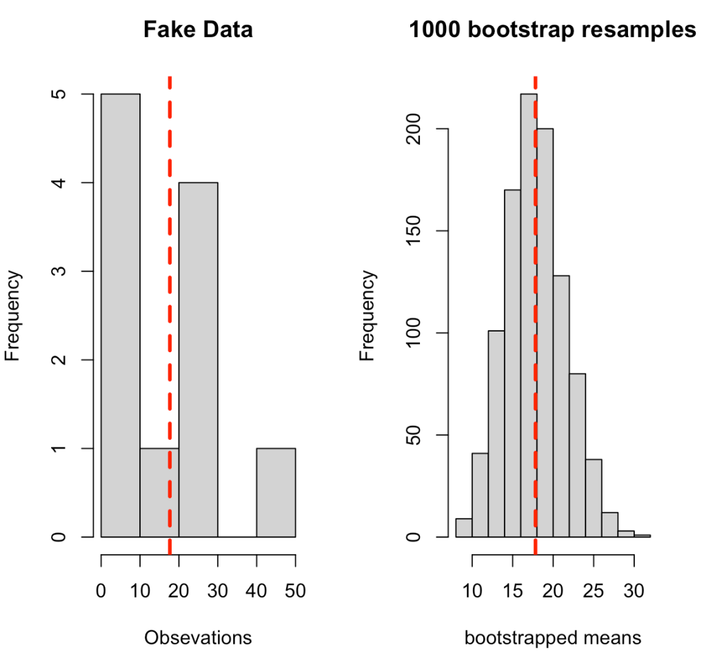
The code below goes through the process of creating some fake data and then writing a for() loop that produces 1000 bootstrap resamples. The for() loop was introduced in Part 1 of this series. In a nutshell, we are taking a random sample from the fake data (with replacement), calculating the mean of that random sample, and storing it in the element boot_dat. From there, we calculate the summary statistics or the original sample and the bootstrap resample, which we store in a data frame for comparison purposes, and then produce a histogram of the original sample and the bootstrap resample, which are visualized below the code.

library(tidyverse)

## create fake data
dat <- c(5, 10, 44, 3, 29, 10, 16.7, 22.3, 28, 1.4, 25)

### Bootstrap Resamples ###
# we want 1000 bootstrap resamples
n_boots <- 1000

## create an empty vector to store our bootstraps
boot_dat <- rep(NA, n_boots)

# set seed for reproducibility
set.seed(786)

# write for() loop for the resampling
for(i in 1:n_boots){
  # random sample of 1:n number of observations in our data, with replacement
  ind <- sample(1:length(dat), replace = TRUE)
  
  # Use the row indexes to select the given values from the vector and calculate the mean
  boot_dat[i] <- mean(dat[ind])
}

# Look at the first 6 bootstrapped means
head(boot_dat)

### Compare Bootstrap data to original data ###
## mean and standard deviation of the fake data
dat_mean <- mean(dat)
dat_sd <- sd(dat)

# standard error of the mean
dat_se <- sd(dat) / sqrt(length(dat))

# 95% confidence interval
dat_ci95 <- paste0(round(dat_mean - 1.96*dat_se, 1), ", ", round(dat_mean + 1.96*dat_se, 1))

# mean an SD of bootstrapped data
boot_mean <- mean(boot_dat)

# the vector is the mean of each bootstrap sample, so the standard deviation of these means represents the standard error
boot_se <- sd(boot_dat)

# to get the standard deviation we can convert the standard error back
boot_sd <- boot_se * sqrt(length(dat))

# 95% quantile interval
boot_ci95 <- paste0(round(boot_mean - 1.96*boot_se, 1), ", ", round(boot_mean + 1.96*boot_se, 1)) ## Put everything together data.frame(data = c("fake sample", "bootstrapped resamples"), N = c(length(dat), length(boot_dat)), mean = c(dat_mean, boot_mean), sd = c(dat_sd, boot_sd), se = c(dat_se, boot_se), ci95 = c(dat_ci95, boot_ci95)) %&gt;%
  knitr::kable()

# plot the distributions
par(mfrow = c(1, 2))
hist(dat,
     xlab = "Obsevations",
     main = "Fake Data")
abline(v = dat_mean,
       col = "red",
       lwd = 3,
       lty = 2)
hist(boot_dat,
     xlab = "bootstrapped means",
     main = "1000 bootstrap resamples")
abline(v = boot_mean,
       col = "red",
       lwd = 3,
       lty = 2)

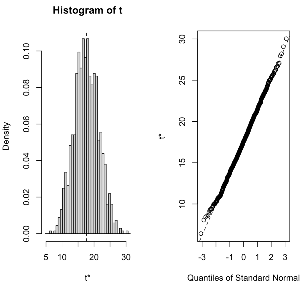
R offers a bootstrap function from the boot package that allows you to do the same thing without writing out your own for() loop. Below is an example of coding the same procedure in the boot package and the outputs the function provides, which are similar to the output we get above, save for slight differences due to random sampling.

# write a function to calculate the mean of our sample data
sample_mean <- function(x, d){
     return(mean(x[d]))
}

# run the boot() function
library(boot)

# run the boot function
boot_func_output <- boot(dat, statistic = sample_mean, R = 1000)

# produce a plot of the output
plot(boot_func_output)

# get the mean and standard error
boot_func_output

# get 95% CI around the mean
boot.ci(boot_func_output, type = "basic", conf = 0.95)

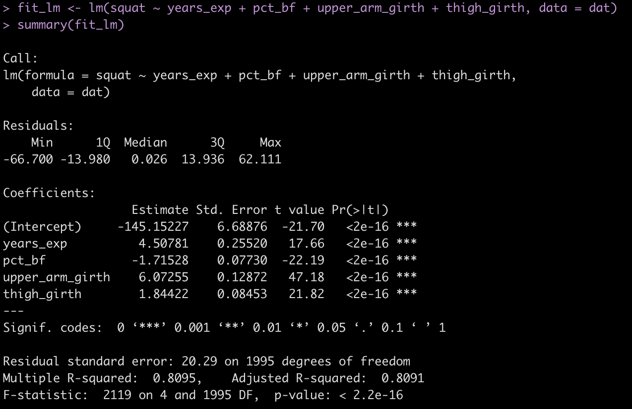
We can bootstrap pretty much anything we want. We don’t have to limit ourselves to producing the distribution around the mean of a population. For example, let’s bootstrap regression coefficients to understand the uncertainty in them.

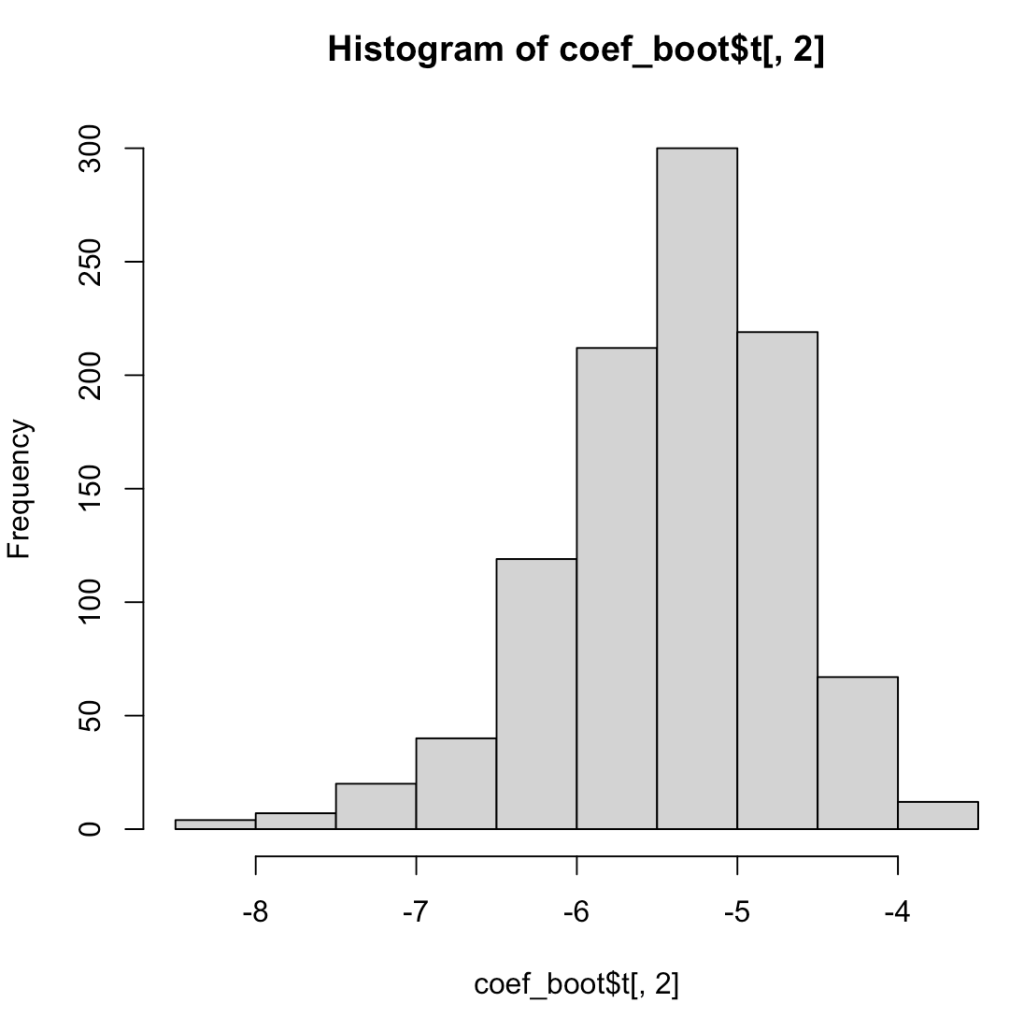
First, let’s use the boot() function to conduct our analysis. We will fit a simple linear regression predicting miles per gallon from engine weight using the mtcars package. We will then write a function for that uses a random sample of rows to create the same linear regression and store those coefficients from 1000 linear regressions so that we can plot a histogram representing the slope coefficient from the resampled models and also summarize the distribution with confidence intervals.

# load the mtcars data
d <- mtcars d %>%
  head()

# fit a regression model
fit_mpg <- lm(mpg ~ wt, data = d)
summary(fit_mpg)
coef(fit_mpg)
confint(fit_mpg)

# Write a function that can perform a bootstrap over the intercept and slope of the model
# bootstrap function
reg_coef_boot <- function(data, row_id){
  # we want to resample the rows
  fit <- lm(mpg ~ wt, data = d[row_id, ])
  coef(fit)
}

# run this once on a small subset of the row ids to see how it works
reg_coef_boot(data = d, row_id = 1:20)

# run the boot() function 1000 times
coef_boot <- boot(data = d, reg_coef_boot, 1000) 

# check the output (coefficient and SE) 
coef_boot 

# get the confidence intervals 
boot.ci(coef_boot, index= 2) 

# all 1000 of the bootstrap resamples can be called coef_boot$t %&gt;%
  head()

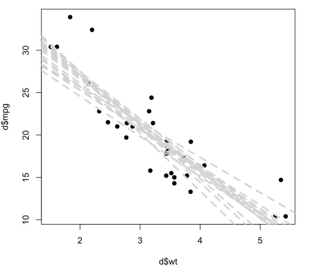
# plot the first 20 bootstrapped intercepts and slopes over the original data
plot(x = d$wt,
     y = d$mpg,
     pch = 19)
for(i in 1:20){
  abline(a = coef_boot$t[i, 1],
       b = coef_boot$t[i, 2],
       lty = 2,
       lwd = 3,
       col = "light grey")
}

## histogram of the slope coefficient
hist(coef_boot$t[, 2])

We can do this by hand if we don’t want to use the built in boot() function. (SIDE NOTE: I usually prefer to code my own resampling and simulations as it gives me more flexibility with respect to the things I’d like to add or the values I’d like to store from each iteration.

Below, instead of producing a histogram of just the slope coefficient, I use both the resampled intercept and slope and add 20 (of the 1000) lines to a scatter plot to show the way in which each of these lines represents a plausible regression line for the data. As you can see, the regression line confidence interval is starting to take shape, even with just 20 out of 1000 resamples, and this gives us a good understanding of not only the variability in our possible regression line fit for the underlying data but also, perhaps should make us less overconfident in our research findings knowing that there are many possible outcomes from the sample data we have obtained.

## 1000 resamples
n_samples <- 1000

## N observations
n_obs <- nrow(mtcars)

## empty storage data frame for the coefficients
coef_storage <- data.frame(
  intercept = rep(NA, n_samples),
  slope = rep(NA, n_samples)
)

for(i in 1:n_samples){
  
  ## sample dependent and independent variables
  row_ids <- sample(1:n_obs, size = n_obs, replace = TRUE)
  new_df <- d[row_ids, ]
  
  ## construct model
  model <- lm(mpg ~ wt, data = new_df)
  
  ## store coefficients
  # intercept
  coef_storage[i, 1] <- coef(model)[1]
  
  # slope
  coef_storage[i, 2] <- coef(model)[2]
  
}

## see results
head(coef_storage)
tail(coef_storage)

## Compare the results to those of the boot function
apply(X = coef_boot$t, MARGIN = 2, FUN = mean)
apply(X = coef_storage, MARGIN = 2, FUN = mean)

apply(X = coef_boot$t, MARGIN = 2, FUN = sd)
apply(X = coef_storage, MARGIN = 2, FUN = sd)

## plot first 20 lines
plot(x = d$wt,
     y = d$mpg,
     pch = 19)
for(i in 1:20){
  abline(a = coef_storage[i, 1],
       b = coef_storage[i, 2],
       lty = 2,
       lwd = 3,
       col = "light grey")
}

Simulating a relationship between two variables

As discussed in Part 1, simulation differs from resampling in that we use the parameters of the observed data to compute a new distribution, versus sampling from the data we have on hand.

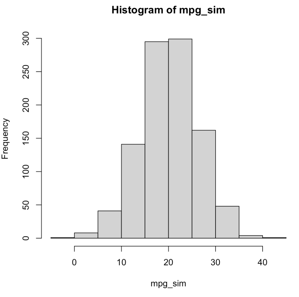
For example, using the mean and standard deviation of mpg from the mtcars data set, we can simulate 1000 random draws from a normal distribution.

## load the mtcars data set
d <- mtcars

## make a random draw from the normal distribution for mph
set.seed(5)
mpg_sim <- rnorm(n = 1000, mean = mean(d$mpg), sd = sd(d$mpg))

## plot and summarize
hist(mpg_sim)

mean(mpg_sim)
sd(mpg_sim)

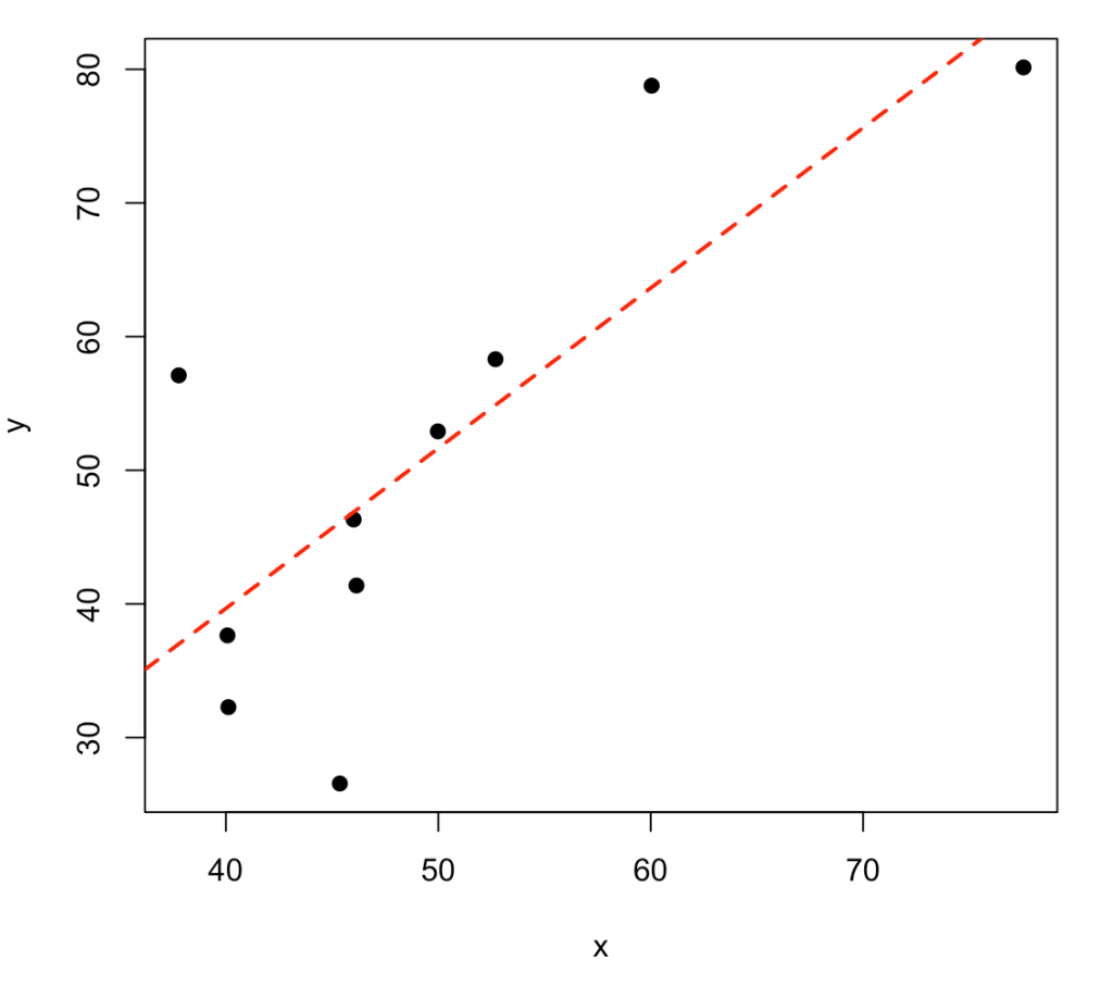
Frequently, we are interested in the relationship between two variables (e.g., correlation, regression, etc.). Let’s simulate two variables, x and y, which are linearly related in some way. To do this, we first simulate the variable x and then simulate y to be x plus some level of random noise.

# simulate x and y
set.seed(1098)
x <- rnorm(n = 10, mean = 50, sd = 10)
y <- x + rnorm(n = length(x), mean = 0, sd = 10)

# put the results in a data frame
dat <- data.frame(x, y)
dat

# how correlated are the two variables
cor.test(x, y)

# fit a regression for the two variables
fit <- lm(y ~ x)
summary(fit)

# plot the two variables with the regression line
plot(x, y, pch = 19)
abline(fit, col = "red", lwd = 2, lty = 2)

Simulating a data set with multiple variables

Frequently, we might have a hypothesis regarding how correlated multiple variables are with each other. The example above produced a relationship of two variables with a direct relationship between them along with some noise. We might want to specify this relationship given a correlation coefficient or covariance between them. Additionally, we might have more than two variables that we want to simulate relationships between.

To do this in R we can take advantage of two packages:

• MASS via the mvrnorm()
• mvtnorm via the mvrnorm()

Both packages have a function for simulating multivariate normal distributions. The primary difference is that the Sigma argument in the MASS package function, mvrnorm(), accepts a covariance matrix while the sigma argument in the mvtnorm package, rmvnorm() accepts a correlation matrix. I’ll show both examples but I tend to stick with the mtvnorm package because (at least for my brain) it is easier for me to think in terms of correlation coefficients instead of covariances.

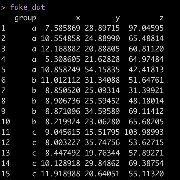
First we simulate some data:

## create fake data
set.seed(1234)
fake_dat <- data.frame(
  group = rep(c("a", "b", "c"), each = 5),
  x = rnorm(n = 15, mean = 10, sd = 2),
  y = rnorm(n = 15, mean = 30, sd = 10),
  z = rnorm(n = 15, mean = 75, sd = 20)
)

fake_dat

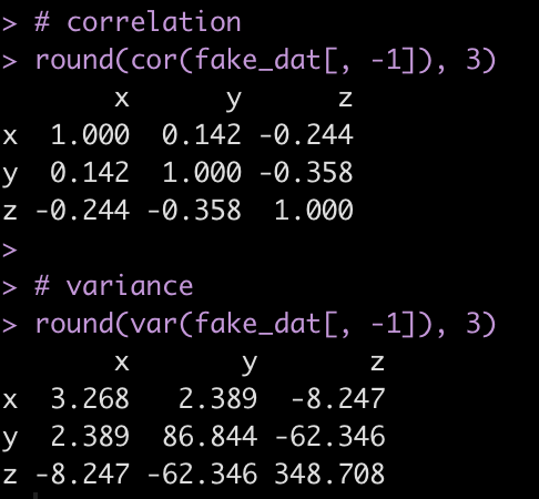
Look at the correlation and variance between the three numeric variables.

# correlation
round(cor(fake_dat[, -1]), 3)

# variance
round(var(fake_dat[, -1]), 3)

We can use this information to simulate new x, y, or z variables.

Simulating x and y with the MASS package

Remember, for the MASS package, the Sigma argument is a matrix of covariances for the variables you are simulating from a multivariate normal distribution.

## get a vector of the mean for each variable
variable_means <- apply(X = fake_dat[, c("x", "y")], MARGIN = 2, FUN = mean)

## Get a matrix of the covariance between x and y
variable_sigmas <- var(fake_dat[, c("x", "y")])

## simulate 1000 new x and y variables using the MASS package
set.seed(98)
new_sim <- MASS::mvrnorm(n = 1000, mu = variable_means, Sigma = variable_sigmas)
head(new_sim)

### look at the results relative to the original x and y
## column means
variable_means
apply(X = new_sim, MARGIN = 2, FUN = mean)

## covariance
var(fake_dat[, c("x","y")])
var(new_sim)

 

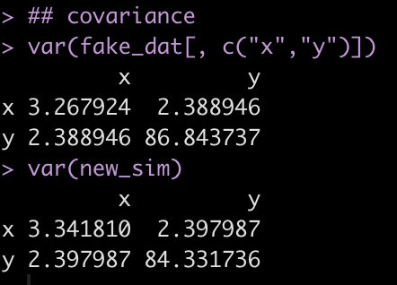
Notice that the variance between x and y (the off diagonal of the matrix) is very similar between the fake data (the observed sample) and the simulated data (new_sim).

Simulating x and y with the mtvnorm package

Different than the MASS package, The rmvnorm() function from the mtvnorm package requires the sigma argument to be a correlations matrix.

Let’s repeat the above process with our fake_dat and simulate a relationship between x and y.

## get a vector of the mean for each variable
variable_means <- apply(X = fake_dat[, c("x", "y")], MARGIN = 2, FUN = mean)

## Get a matrix of the correlation between x and y
variable_cor <- cor(fake_dat[, c("x", "y")])

## simulate 1000 new x and y variables using the mvtnorm package
set.seed(98)
new_sim <- mvtnorm::rmvnorm(n = 1000, mean = variable_means, sigma = variable_cor)
head(new_sim)

### look at the results relative to the original x and y
## column means
variable_means
apply(X = new_sim, MARGIN = 2, FUN = mean)

## correlation
cor(fake_dat[, c("x","y")])
cor(new_sim)

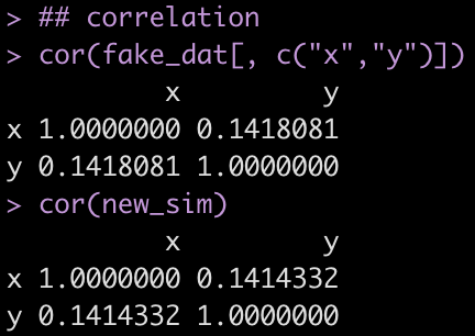
Similar to the previous example, we notice that the off diagonal correlation coefficient between x and y is very similar when comparing the simulated data to the fake data.

So, what is happening here? Both packages produce the same result, one uses a covariance matrix and the other uses a correlation matrix. The kicker here is understanding the relationship between covariance and correlation. Covariance is explaining how two variables vary together, however, its units aren’t on a scale that is directly interpretable to us. But, we can convert the covariance between two variables to a correlation by dividing their covariance by the product of their individual standard deviations.

For example, here is the covariance matrix between x and y in the fake data set.

cov(fake_dat[, c("x", "y")])

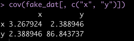
The covariance between the two variables is on the off diagonal, 2.389. We can store this in its own element.

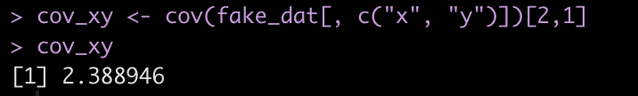
cov_xy <- cov(fake_dat[, c("x", "y")])[2,1]
cov_xy

Let’s store the standard deviation of both `x` and `y` in their own elements to make the equation easier to read.

sd_x <- sd(fake_dat$x)
sd_y <- sd(fake_dat$y)

Finally, we calculate the correlation by dividing the covariance by the product of the two standard deviations and check our results by calling the cor() function on the two variables.

## covariance to correlation
cov_to_cor <- cov_xy / (sd_x * sd_y)
cov_to_cor

## check results with the corr() function
cor(fake_dat[, c("x", "y")])

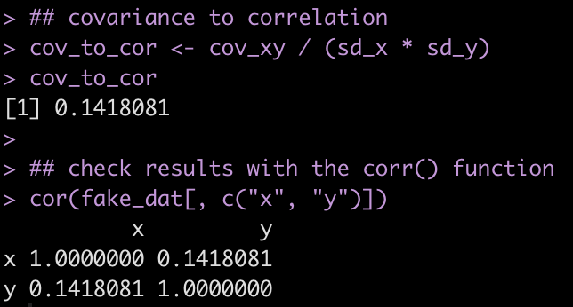
By dividing the covariance by the product of the standard deviation of the two variables we can see the relationship between covariance and correlation and now understand why the results from the MASS and mtvnorm produce similar results. Understanding this relationship becomes valuable when we move onto simulating more complex relationships, for example when simulating mixed models.

What about three variables?

What if we want to simulate all three variables — x, y, and z?

All we need is a larger covariance or correlation matrix, depending on which of the above packages you’d like to use. Since we usually won’t be creating these matrices from a data set, as I did above, I’ll show how to create your own matrix and run the simulation.

First, let’s store a vector of plausible mean values for x, y, and z.

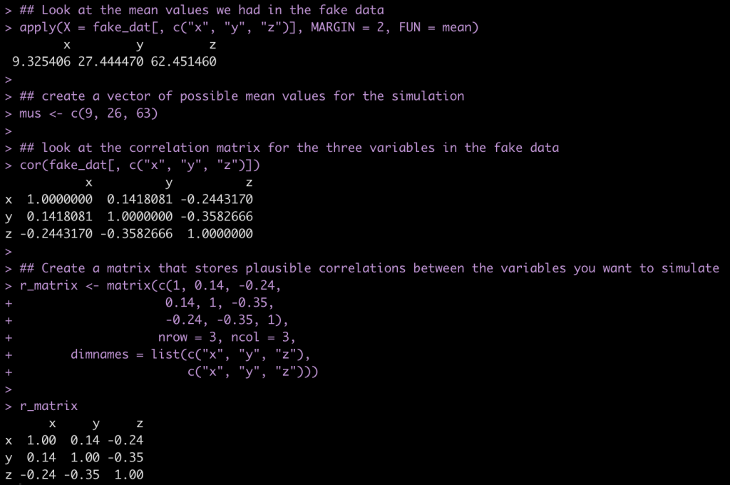
## Look at the mean values we had in the fake data
apply(X = fake_dat[, c("x", "y", "z")], MARGIN = 2, FUN = mean)

## create a vector of possible mean values for the simulation
mus <- c(9, 26, 63)

## look at the correlation matrix for the three variables in the fake data
cor(fake_dat[, c("x", "y", "z")])

## Create a matrix that stores plausible correlations between the variables you want to simulate
r_matrix <- matrix(c(1, 0.14, -0.24,
                    0.14, 1, -0.35,
                    -0.24, -0.35, 1), 
                   nrow = 3, ncol = 3,
       dimnames = list(c("x", "y", "z"),
                       c("x", "y", "z")))

r_matrix

Next, we create 1000 simulations of a multivariate normal distribution between x, y, and z. We then compare our correlation coefficients between the fake data, which is our observed sample, and the simulated data

## simulate 1000 new x, y, and z variables using the mvtnorm package
set.seed(43)
new_sim <- mvtnorm::rmvnorm(n = 1000, mean = mus, sigma = r_matrix)
head(new_sim)

### look at the results relative to the original x, y, and z
## column means
apply(X = fake_dat[, c("x", "y", "z")], MARGIN = 2, FUN = mean)
apply(X = new_sim, MARGIN = 2, FUN = mean)

## correlation
cor(fake_dat[, c("x", "y", "z")])
cor(new_sim)

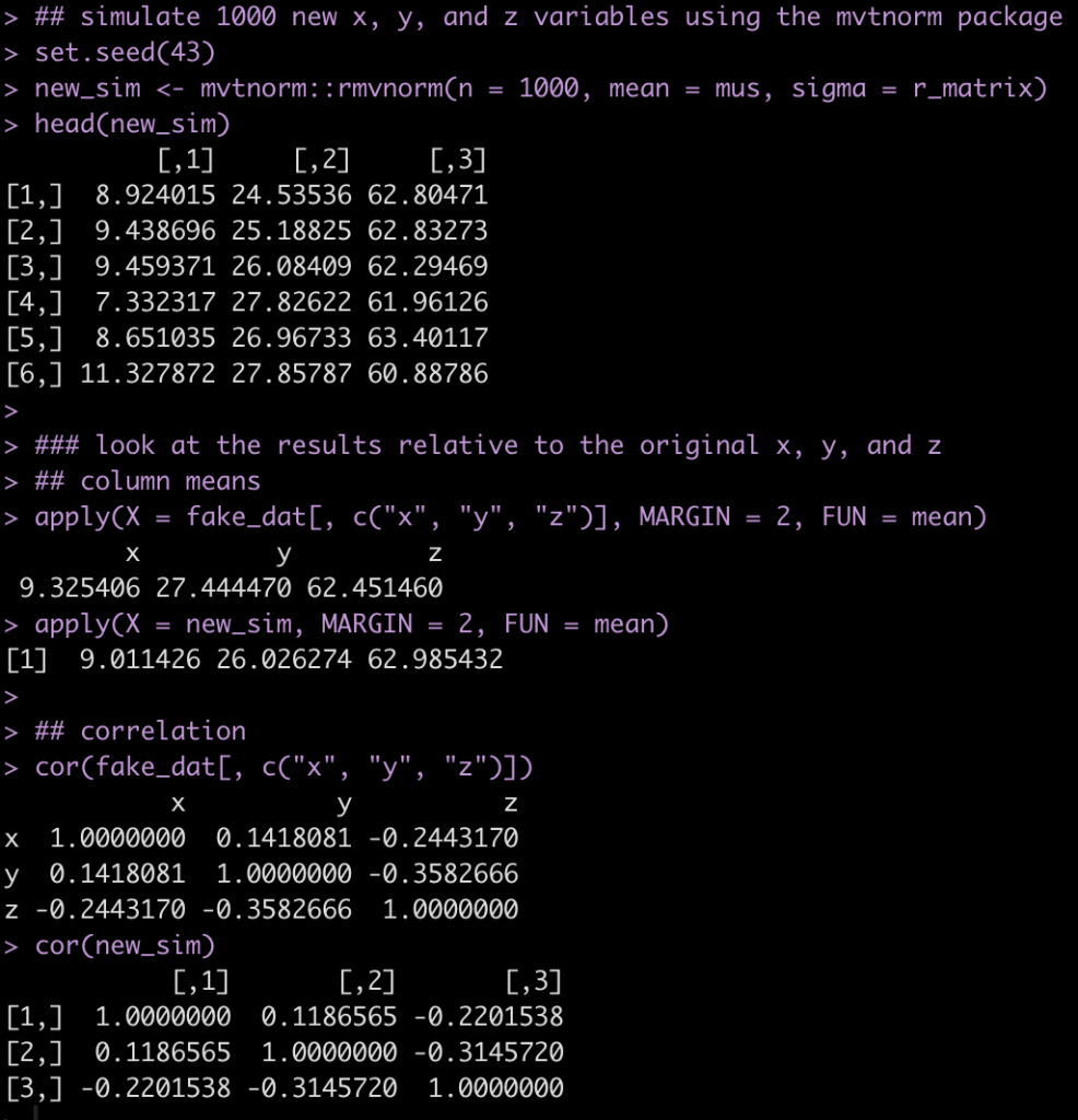
The results from the simulation are pretty similar to the fake_dat dataset. If you recall from the correlation matrix and the vector of means, we didn’t use exact values from the observed data, so that, along with the random draws from the multivariate normal distribution, leads to the small amount of differences.

Wrapping Up

In this second installment of the Simulations in R series we’ve walked through how to code our own bootstrap resampling for both means and regression coefficients. We then progressed to building simulations of both bivariate and multivariate normal distributions. This, along with the basic info in Part 1, will serve us well as we progress forward in our work and begin to explore using simulations for comparisons between group means (simulated t-tests) and building regression models.

As always, all of the code is available in the Github repository.

I’ve talked a lot in this blog about making predictions (see HERE, HERE, and HERE) as well as the difference between confidence intervals and prediction intervals and why you’d use one over the other (see HERE). Tonight I was having a discussion with a colleague about some models he was working on and he was building some confidence intervals around his predictions. That got me to thinking about the various ways we can code confidence intervals, quantile intervals, and prediction intervals in R. So, I decided to put together this quick tutorial to provide a few different ways of constructing these values (after all, unless we can calculate the uncertainty in our predictions, point estimate predictions are largely useless on their own).

The full code is available on my GITHUB page.

Load packages, get data, and fit regression model

The only package we will need is {tidyverse}, the data will be the mtcars dataset and the model will be a linear regression which attempts to predict mpg from wr and carb.

## Load packages
library(tidyverse)

theme_set(theme_classic())

## Get data
d <- mtcars d %>%
  head()

## fit model
fit_lm <- lm(mpg ~ wt + carb, data = d)
summary(fit_lm)

Get some data to make predictions on

We will just grab a random sample of 5 rows from the original data set and use that to make some predictions on.

## Get a few rows to make predictions on
set.seed(1234)
d_sample <- d %>%
  sample_n(size = 5) %>%
  select(mpg, wt, carb)

d_sample

Confidence Intervals with the predict() function

Using preidct() we calculate the predicted value with 95% Confidence Intervals.

## 95% Confidence Intervals
d_sample %>%
  bind_cols(
    predict(fit_lm, newdata = d_sample, interval = "confidence", level = 0.95)
  )

Calculate confidence intervals by hand

Instead of using the R function, we can calculate the confidence intervals by hand (and obtain the same result).

## Calculate the 95% confidence interval by hand
level <- 0.95
alpha <- 1 - (1 - level) / 2
t_crit <- qt(p = alpha, df = fit_lm$df.residual) 

d_sample %>%
  mutate(pred = predict(fit_lm, newdata = .),
         se_pred = predict(fit_lm, newdata = ., se = TRUE)$se.fit,
         cl95 = t_crit * se_pred,
         lwr = pred - cl95,
         upr = pred + cl95)

Calculate confidence intervals with the qnorm() function

Above, we calculated a 95% t-critical value for the degrees of freedom of our model. Alternatively, we could calculate 95% confidence intervals using the standard z-critical value for 95%, 1.96, which we obtain with the qnorm() function.

d_sample %>%
  mutate(pred = predict(fit_lm, newdata = .),
         se_pred = predict(fit_lm, newdata = ., se = TRUE)$se.fit,
         lwr = pred + qnorm(p = 0.025, mean = 0, sd = 1) * se_pred,
         upr = pred + qnorm(p = 0.975, mean = 0, sd = 1) * se_pred)

Calculate quantile intervals via simulation

Finally, we can calculate quantile intervals by simulating predictions using the predicted value and standard error for each of the observations. We simulate 1000 times from a normal distribution and then use the quantile() function to get our quantile intervals.

If all we care about is a predicted value and the lower and upper intervals, we can use the rowwise() function to indicate that we are going to do a simulation for each row and then store the end result (our lower and upper quantile intervals) in a new column.

## 95% Quantile Intervals via Simulation
d_sample %>%
  mutate(pred = predict(fit_lm, newdata = .),
         se_pred = predict(fit_lm, newdata = ., se = TRUE)$se.fit) %>%
  rowwise() %>%
  mutate(lwr = quantile(rnorm(n = 1000, mean = pred, sd = se_pred), probs = 0.025),
         upr = quantile(rnorm(n = 1000, mean = pred, sd = se_pred), probs = 0.975))

While that is useful, there might be times where we want to extract the full simulated distribution. We can create a simulated distribution (1000 simulations) for each of the 5 observations using a for() loop.

## 95% quantile intervals via Simulation with full distribution
N <- 1000
pred_sim <- list()

set.seed(8945)
for(i in 1:nrow(d_sample)){
  
  pred <- predict(fit_lm, newdata = d_sample[i, ])
  se_pred <- predict(fit_lm, newdata = d_sample[i, ], se = TRUE)$se.fit
  
  pred_sim[[i]] <- rnorm(n = N, mean = pred, sd = se_pred)
  
}

sim_df <- tibble( sample_row = rep(1:5, each = N), pred_sim = unlist(pred_sim) ) 

sim_df %>%
  head()

Next we summarize the simulation for each observation.

# get predictions and quantile intervals
sim_df %>%
  group_by(sample_row) %>%
  summarize(pred = mean(pred_sim),
         lwr = quantile(pred_sim, probs = 0.025),
         upr = quantile(pred_sim, probs = 0.975)) %>%
  mutate(sample_row = rownames(d_sample))

We can then plot the entire posterior distribution for each observation.

# plot the predicted distributions
sim_df %>%
  mutate(actual_value = rep(d_sample$mpg, each = N),
         sample_row = case_when(sample_row == 1 ~ "Hornet 4 Drive",
                                sample_row == 2 ~ "Toyota Corolla",
                                sample_row == 3 ~ "Honda Civic",
                                sample_row == 4 ~ "Ferrari Dino",
                                sample_row == 5 ~ "Pontiac Firebird")) %>%
  ggplot(aes(x = pred_sim)) +
  geom_histogram(color = "white",
                 fill = "light grey") +
  geom_vline(aes(xintercept = actual_value),
             color = "red",
             size = 1.2,
             linetype = "dashed") +
  facet_wrap(~sample_row, scale = "free_x") +
  labs(x = "Predicted Simulation",
       y = "count",
       title = "Predicted Simulation with actual observation (red line)",
       subtitle = "Note that the x-axis are specific to that simulation and not the same")

Prediction Intervals with the predict() function

Next we turn attention to prediction intervals, which will be wider than the confidence intervals because they are incorporating additional uncertainty.

The predict() function makes calculating prediction intervals very convenient.

## 95% Prediction Intervals
d_sample %>%
  bind_cols(
    predict(fit_lm, newdata = d_sample, interval = "predict", level = 0.95)
  )

Prediction Intervals from a simulated distribution

Similar to how we simulated a distribution for calculating quantile intervals, above, we will perform the same procedure here. The difference is that we need to get the residual standard error (RSE) from our model as we need to add this additional piece of uncertainty (on top of the predicted standard error) to each of the simulated predictions.

## 95% prediction intervals from a simulated distribution 
# store the model residual standard error
sigma <- summary(fit_lm)$sigma

# run simulation
N <- 1000
pred_sim2 <- list()

set.seed(85)
for(i in 1:nrow(d_sample)){
  
  pred <- predict(fit_lm, newdata = d_sample[i, ])
  se_pred <- predict(fit_lm, newdata = d_sample[i, ], se = TRUE)$se.fit
  
  pred_sim2[[i]] <- rnorm(n = N, mean = pred, sd = se_pred) + rnorm(n = N, mean = 0, sd = sigma)
  
}

# put results in a data frame
sim_df2 <- tibble( sample_row = rep(1:5, each = N), pred_sim2 = unlist(pred_sim2) ) 

sim_df2 %>%
  head()

We summarize our predictions and their intervals.

# get predictions and intervals
sim_df2 %>%
  group_by(sample_row) %>%
  summarize(pred = mean(pred_sim2),
            lwr = quantile(pred_sim2, probs = 0.025),
            upr = quantile(pred_sim2, probs = 0.975)) %>%
  mutate(sample_row = rownames(d_sample))

Finally, we plot the simulated distributions for each of the observations.

Wrapping Up

Uncertainty is important to be aware of and convey whenever you share your predictions. The point estimate prediction is one a single value of many plausible values given the data generating process. This article provided a few different approaches for calculating uncertainty intervals. The full code is available on my GITHUB page.