Introduction
The collection of serial measurements on athletes across a season (or multiple seasons) is one of the more common types of data being generated in the applied sport science environment. The question that coaches and practitioners often have is, “Is this player outside of their ‘normal range’?”
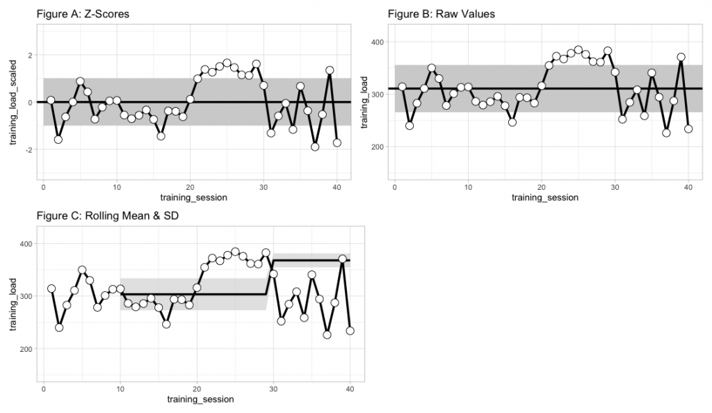
The best approach for establishing a reference range of ‘normal’ values is a frequently discussed topic in sport science. One common strategy is to use z-scores and represent the reference range as 1 standard deviation above or below the mean (Figure A) or plot the raw values and set the reference range 1 standard deviation above or below the raw mean (Figure B), for practitioners who might have a difficult time understanding standardized scores. Of course, the mean and standard deviation will now be related to all prior values. As such, if the athletes go through a training phase with substantially higher values than other phases (e.g., training camp) it could skew your reference ranges. To alleviate this issue, some choose to use a rolling mean and standard deviation, to represent the normal range of values relative to more recent training sessions (Figure C).
A problem with the approaches above is that they require a number of training sessions to allow a mean and standard deviation to be determined for the individual athlete. One solution to this issue is to base our initial normal reference ranges off of prior knowledge that we have from collecting data on players in previous seasons (or prior knowledge from research papers, if we don’t have data of our own yet). This type of Bayesian updating approach has been applied in WADA’s drug testing practices1. More recently, Hecksteden et al., used this approach to evaluate the CK levels of team-sport athletes in both fatigued and non-fatigued states2.
The mathematics of the approach was presented in the paper but might look intimidating to those not used to looking at mathematical equations in this manner. 

The author’s provided a nice excel sheet where you can input your own data and get the updated reference ranges. However, the sheet is a protected sheet, which doesn’t afford the opportunity of seeing how the underlying equations work and you can’t alter the sheet to make appropriate for your data (for example, the data in the sheet log transforms the raw data automatically). Thus, I’ve decided to code the analysis out, both in excel and R, to help practitioners looking to adopt this approach.
Setting Priors
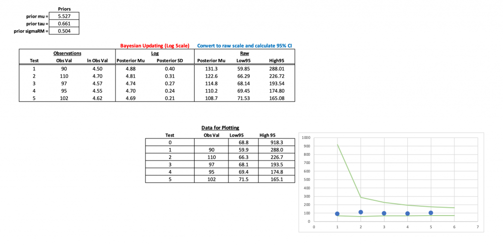
To apply this type of analysis, we need to first establish some prior values for three parameters: Prior Mean (mu), Prior Standard Deviation (tau), and a Prior Repeated-Measures Standard Deviation (sigmaRM). These values represent our current knowledge of the variable we are measuring before seeing any new data. As new data is collected, we can update these priors to get an individual (posterior) estimate for the athlete. I’ll use the priors set by Hecksteden and colleagues for CK levels of Male athletes:
- Mu = 5.527
- Tau = 0.661
- sigmaRM = 0.504
Once we have established our prior parameters, we are ready to update them, using the math equations above, as new data comes in.
Bayesian Updating in Excel
The excel sheet is available at my GitHub page. It looks like this:
All of the heavy lifting occurs in the two columns under the header Bayesian Updating (Log Scale). The equation in the first row (Test 1) is different than the other equations below it because requires the prior information to get going. After that first test, the updated data become the prior for the next test and this continues for all tests forward. You can download the excel sheet and see how the equations work, so I won’t go through them here. Instead, I’ll show them more clearly in the R script, below.
Bayesian Updating in R
We first need to convert the math equations provided in the paper (posted above) into R code. Rather that leaving things to mathematical notation, I’ll plug in the variables in plain English:
To be clear, here are the definitions for the variables above:
Now that we know the variables we need for each equation we can begin the process of updating or reference ranges.
First create a data set of the test observations and their log values. This will be the same data we observed in our excel sheet:
Then we set our priors (in log format):
## priors
prior_mu <- 5.527
prior_sd <- 0.661
prior_repeated_measure_sd <- 0.504
We will start by seeing how the updating works for the mean and standard deviation parameters after the first test. To do this, we will create a function for each parameter (mean and standard deviation) that updates the priors with the observed values based on the above equations:
posterior_mu <- function(prior_mu, prior_sd, prior_repeated_measure_sd, obs_value){

  numerator <- prior_repeated_measure_sd^2 * prior_mu + prior_sd^2 * obs_value
  denominator <- prior_repeated_measure_sd^2 + prior_sd^2

  post_mu <- numerator / denominator
  return(post_mu)

  }

posterior_sd <- function(prior_repeated_measure_sd, prior_sd, test_num){

  post_var <- 1 / ((test_num - 1 + 1) * 1/prior_repeated_measure_sd^2 + 1/prior_sd^2)
  post_sd <- sqrt(post_var)
  return(post_sd)

}
After running the functions on the observations of our first test, our updated mean and standard deviation are:

Notice that we obtain the same values that we see following test_1 in our excel workbook. We can also calculate 95% confidence intervals and take the exponent (since the data is on a log scale) to get the individual athlete’s updated reference range on the raw scale:
 Again, these results confirm the values we see in our excel workbook.
That’s cool and all, but we need to be able to iteratively update the data set as new data comes in. Let’s write a for() loop!
First, we create a new column in the data that provides us with the updated standard deviation after observing the results in each test. This is a necessary first step as we will use this value to then update the mean value.
## Calculate the updated SD based on sample size
df2 <- df %>%
  mutate(bayes_sd = sqrt(1 / ((test - 1 + 1) * 1 / prior_repeated_measure_sd^2 + 1 / prior_sd^2)))

df2
Next, we need a for() loop. This is a bit tricky because test_1 is updating based solely on the priors while all other tests (test_2 to test_N) will be updating based on the mean and standard deviation in the row above them. Thus, we need to have our for() loop look back at the previous row above it once those values are calculated. This sort of thing is easy to set up in excel but in R (or Python) we need to think about how to code our row indexes. I covered this sort of iterative row computing in two previous articles HERE and HERE.
Within the loop we first set up vectors for the prior variance (sd^2), the denominator in our equation, and the log transformed observations from our data set. Then, we calculate the updated posterior for the mean (mu) on each pass through the loop, each time using the value preceding it in the vector, [i – 1], to allow us to iteratively update the data.
Once we run the loop, we add the results to our data set (removing the first observation in the vector since that was the original prior before seeing any data):
# Create a vector to store results
N <- length(df2$ln_value) + 1
bayes_mu <- c(prior_mu, rep(NA, N - 1))


## For loop
for(i in 2:N){

  ## Set up vectors for the variance, denominator, and newly observed values
  prior_var <- c(prior_sd^2, df2$bayes_sd^2)
  denominator <- prior_repeated_measure_sd^2 + prior_var
  vals <- df2$ln_value

  ## calculate bayesian updated mu
  bayes_mu[i] <- (prior_repeated_measure_sd^2 * bayes_mu[i-1] + prior_var[i-1] * vals[i-1]) / denominator[i-1]

}

df2$bayes_mean <- bayes_mu[-1]
df2
The two columns, bayes_sd and bayes_mean, contain our updated prior values and they are the exact same results we obtained in our excel workbook.
To use these updated parameters for creating individual athlete reference ranges, we calculate the 95% Confidence Intervals:
NOTE: I added a row at the start of data frame to establish the priors, before seeing the data, so that they could also be plotted as part of the reference ranges.
### Confidence Intervals
first_prior <- data.frame(test = 0, value = NA, ln_value = NA, bayes_sd = prior_sd, bayes_mean = prior_mu)

df2 <- df2 %>%
  bind_rows(first_prior) %>%
  arrange(test)

## Exponentiate back to get the reference range
df2$low95 <- exp(df2$bayes_mean - 1.96*df2$bayes_sd)
df2$high95 <- exp(df2$bayes_mean + 1.96*df2$bayes_sd)
df2
Finally, we plot the observations along with the continually updated references ranges. You can clearly see how large the normal range is before seeing any data (test_0) and then how quickly this range begins to shrink down once we start observing data from the individual.
To access the R code and the excel workbook please visit my GitHub page.
References
- Sottas PE et al. (2007). Bayesian detection of abnormal values in longitudinal biomarkers with application to T/E ratio. Biostatistics; 8(2): 285-296.
- Hecksteden et al. (2017). A new method to individualize monitoring of muscle recovery in athletes. Int J Sport Phys Perf; 12: 1137-1142.


