For the next installment of our simulation blog series we will use simulation to look at the Multicollinearity assumption in linear regression.
For a refresher, here are the previous 5 articles in this series:
- Part 1 discussed the basic functions for simulating and sampling data in R.
- Part 2 walked us through how to perform bootstrap resampling and then simulate bivariate and multivariate distributions.
- Part 3 we worked making group comparisons by simulating thousands of t-tests
- Part 4 building simulations for linear regression
- Part 5 using simulation to investigate the homoskedasticity assumption in regression.
The entire code for this series is accessible on my GITHUB page.
Multicollinearity
Multicollinearity occurs when two independent variables in a regression model are highly correlated with each other. Such a situation can produce problems with interpretation of the beta coefficients of the model, may increase standard errors in the model, and can lead to over fitting of the data. We can simulate this issue in order to get a better understanding of how multicollinearity can influence a regression model.
Constructing the simulation
We will use the mvnorm package to help us construct a simulation where the two independent variables share a certain level of correlation between each other.
First, we will create the true model parameters: an intercept of 2, a beta1 of 5, and a beta2 of 10. We also create a vector of correlation coefficients from 0 to 0.99 and a few data frames to store the results of our model. We will also specify that at each correlation coefficient we want 200 random draws from the multivariate normal distribution.
## load packages
library(tidymodels)
library(patchwork)
library(mvtnorm)

set.seed(999)

# create the true model parameters
intercept <- 2
beta1 <- 5
beta2 <- 10

## Number of draws from a multivariate normal distribution
n <- 200

## Create a data frame to store model results
sim_params <- data.frame(intercept = NA,
                      intercept_se = NA,
                      beta1 = NA,
                      beta1_se = NA,
                      beta2 = NA,
                      beta2_se = NA,
                      model_rse = NA)

## create levels of multicollinearity between the two independent variables
cor_coefs <- c(seq(from = 0, to = 0.9, by = 0.1), 0.99)

# data frame to store the average beta coefficient and their standard deviations form the simulation
mean_betas <- data.frame(beta1 = NA,
                       sd_beta1 = NA,
                       beta2 = NA,
                       sd_beta2 = NA)
Next, we will create a nested for() loop to construct out simulations.
- The outer part of the loop begins by creating the multivariate normal distribution. We use the rmvnorm(), which means we first specify a correlation matrix using our vector of correlation coefficients we specified above. Once we have the two correlated variables we can put them into the inner loop.
- The inner loop is where we create a regression equation for the given correlation between the two variables. We create 100 regression simulations for each correlation coefficient.
- Once the inner loop is finished running we store the results at the bottom of the outer loop. Instead of storing all of the results, we take the average of the 100 beta coefficients and their respective standard errors for each correlation coefficient.
## loop
for(j in 1:length(cor_coefs)){

  ## Create a correlation matrix between beta1 and beta2
  beta_corr <- matrix(c(1, cor_coefs[j], cor_coefs[j], 1), nrow = 2, ncol = 2)

  ## create a multivariate normal distribution
  cor_df <- rmvnorm(n = n, mean = c(0, 0), sigma = beta_corr)
  X1 <- cor_df[, 1]
  X2 <- cor_df[, 2]

  ## simulate 100 regression simulations
  for(i in 1:100){

    # set up the model
    y_hat <- intercept + beta1*X1 + beta2*X2 + rnorm(n = n, mean = 0, sd = 1)

    # construct a regression equation
    model <- lm(y_hat ~ X1 + X2)

    # store the variance-covariance matrix
    vcv <- vcov(model)

    # estimates for the intercept
    sim_params[i, 1] <- model$coef[1]

    # estimates for the beta1
    sim_params[i, 3] <- model$coef[2]

    # estimates for beta2
    sim_params[i, 5] <- model$coef[3]

    # SE for the intercept
    sim_params[i, 2] <- sqrt(diag(vcv)[1])

    # SE for beta1
    sim_params[i, 4] <- sqrt(diag(vcv)[2])

    # SE for beta2
    sim_params[i, 6] <- sqrt(diag(vcv)[3])

    # model RSE
    sim_params[i, 7] <- summary(model)$sigma
  }

  mean_betas[j, ] <- c(mean(sim_params[, 3]), mean(sim_params[, 4]), mean(sim_params[, 5]), mean(sim_params[, 6]))

}
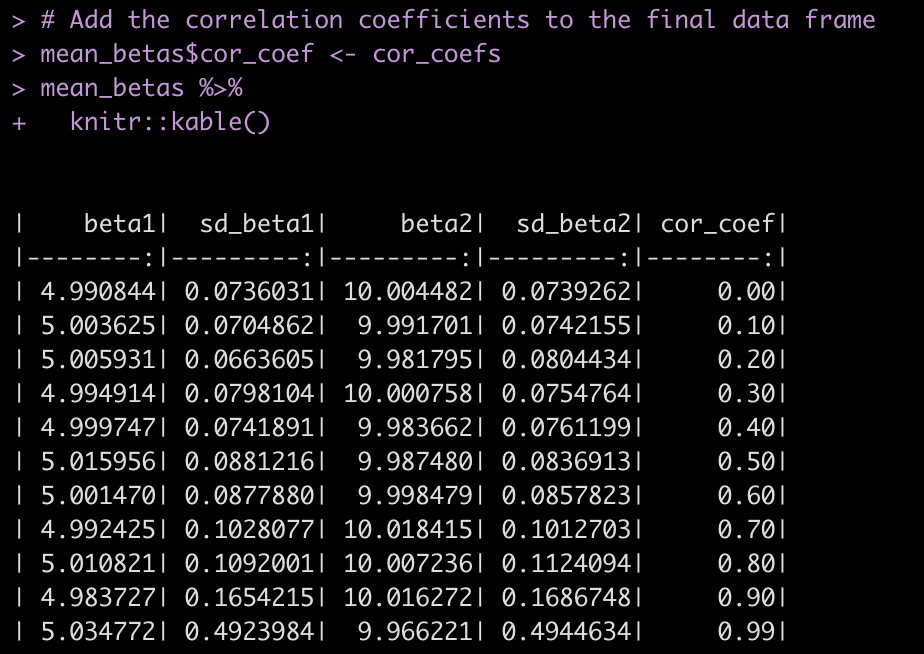
The final result is a data frame with 10 rows, one for each correlation coefficient and the average of 100 regression simulations for the beta coefficients and their standard errors.
# Add the correlation coefficients to the final data frame
mean_betas$cor_coef <- cor_coefs mean_betas %>%
  knitr::kable()
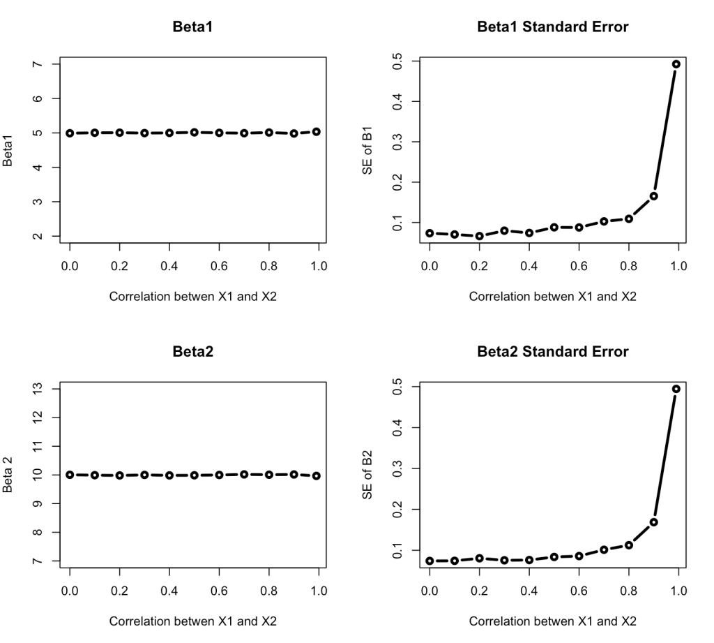
Finally, we plot each of the results with the correlation coefficients on the x-axis.
# Plot the results
par(mfrow = c(2,2))
plot(x = mean_betas$cor_coef,
     y = mean_betas$beta1,
     main = "Beta1",
     lwd = 3,
     type = "b",
     ylim = c(2, 7),
     xlab = "Correlation betwen X1 and X2",
     ylab = "Beta1")
plot(x = mean_betas$cor_coef,
     y = mean_betas$sd_beta1,
     main = "Beta1 Standard Error",
     lwd = 3,
     type = "b",
     xlab = "Correlation betwen X1 and X2",
     ylab = "SE of B1")
plot(x = mean_betas$cor_coef,
     y = mean_betas$beta2,
     main = "Beta2",
     lwd = 3,
     type = "b",
     ylim = c(7, 13),
     xlab = "Correlation betwen X1 and X2",
     ylab = "Beta 2")
plot(x = mean_betas$cor_coef,
     y = mean_betas$sd_beta2,
     main = "Beta2 Standard Error",
     lwd = 3,
     type = "b",
     xlab = "Correlation betwen X1 and X2",
     ylab = "SE of B2")
The beta coefficients themselves remain relatively unchanged in our simulation across the various correlations levels. However, once the correlation between the two independent variables reaches about 0.7 the standard errors around the beta coefficients begin to increase exponentially, increasing our uncertainty about the true parameter values.
Wrapping Up
We’ve now covered using simulation to investigate two assumptions of linear regression. Our next installment will investigate another linear regression assumption before we proceed on to simulating other types of models.
For the full code, check out my GITHUB page.


