Yesterday, I talked about how t-test and ANOVA are fundamentally just linear regression. But what about something more complex? What about something like a neural network?
Whenever people bring up neural networks I always say, “The most basic neural network is a sigmoid function. It’s just logistic regression!!” Of course, neural networks can get very complex and there is a lot more than can be added to them to maximize their ability to do the job. But fundamentally, they look like regression models and when you add several hidden layers (deep learning) you end up just stacking a bunch of regression models on top of each other (I know I’m over simplifying this a little bit).
Let’s see if we can build a simple neural network to prove it. As always, you can access the full code on my GITHUB page.
Loading packages, functions, and data
We will load {tidyverse} for data cleaning, {neuralnet} for building our neural network, and {mlbench} to access the Boston housing data.
I create a z-score function that will be used to standardize the features for our model. We will keep this simple and attempt to predict Boston housing prices (mdev) using three features (rm, dis, indus). To read more about what these features are, in your R console type ?BostonHousing. Once we’ve selected those features out of the data set, we apply our z-score function to them.
## Load packages
library(tidyverse)
library(neuralnet)
library(mlbench)

## z-score function
z_score <- function(x){
  z <- (x - mean(x, na.rm = TRUE)) / sd(x, na.rm = TRUE)
  return(z)
}

## get data
data("BostonHousing")

## z-score features
d <- BostonHousing %>%
  select(medv, rm, dis, indus) %>%
  mutate(across(.cols = rm:indus,
                ~z_score(.x),
                .names = "{.col}_z"))

d %>%
  head()
Train/Test Split
There isn’t much of a train/test split here because I’m not building a full model to be tested. I’m really just trying to show how a neural network works. Thus, I’ll select the first row of data as my “test” set and retain the rest of the data for training the model.
## remove first observation for making a prediction on after training
train <- d[-1, ]
test <- d[1, ]
Neural Network Model
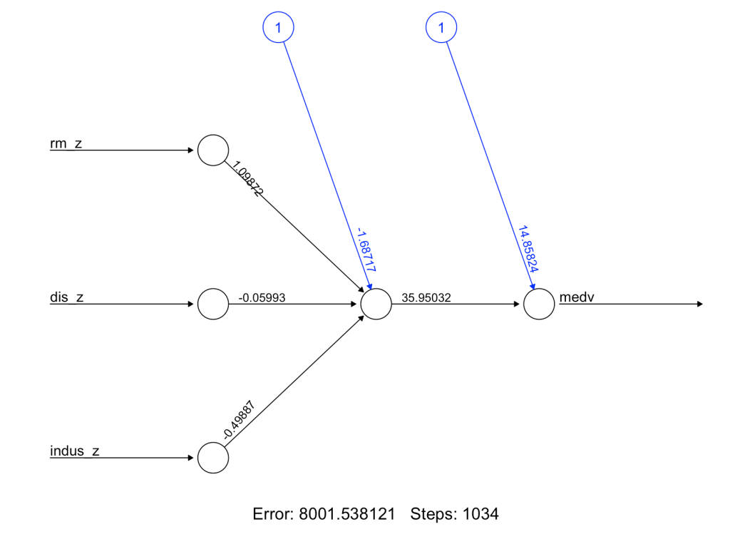
We build a simple model with 1 hidden layer and then plot the output. In the plot we see various numbers. The numbers in black refer to our weights and the numbers in blue refer to the biases.
## Simple neural network with one hidden layer
set.seed(9164)
fit_nn <- neuralnet(medv ~ rm_z + dis_z + indus_z,
                    data = train,
                    hidden = 1,
                    err.fct = "sse",
                    linear.output = TRUE)

## plot the neural network
plot(fit_nn)
Making Predictions — It’s linear regression all the way down!
As stated above, we have weights (black numbers) and biases (blue numbers). If we are trying to frame up the neural network as being a bunch of stacked together linear regressions then we can think about the weights as functioning like regression coefficients and the biases functioning like the linear model intercept.
Let’s take each variable from the plot and store them in their own elements so that we can apply them directly to our test observation and write out the equation by hand.
## Predictions are formed using the weights (black) and biases
# Store the weights and biases from the plot and put them into their own elements
rm_weight <- 1.09872
dis_weight <- -0.05993
indus_weight <- -0.49887

# There is also a bias in the hidden layer
hidden_weight <- 35.95032

bias_1 <- -1.68717
bias_2 <- 14.85824
With everything stored, we are ready to make a prediction on the test observations
We begin at the input layer by multiplying each z-scored value by the corresponding weight from the plot above. We sum those together and add in the first bias — just like we would with a linear regression.
# Start by applying the weights to their z-scored values, sum them together and add
# in the first bias
input <- bias_1 + test$rm_z * rm_weight + test$dis_z * dis_weight + test$indus_z * indus_weight
input
One regression down, one more to go! But before we can move to the next regression, we need to transform this input value. The neural network is using a sigmoid function to make this transformation as the input value moves through the hidden layer. So, we should apply the sigmoid function before moving on.
# transform input -- the neural network is using a sigmoid function
input_sig <- 1/(1+exp(-input))
input_sig

We take this transformed input and multiply it by the hidden weight and then add it to the second bias. This final regression equation produces the predicted value of the home.
prediction <- bias_2 + input_sig * hidden_weight
prediction

The prediction here is in the thousands, relative to census data from the 1970’s.
Let’s compare the prediction we got by hand to what we get when we run the predict() function.
## Compare the output to what we would get if we used the predict() function
predict(fit_nn, newdata = test)
Again, if you’d like the full code, you can access it on by GITHUB page.
Wrapping Up
Yesterday we talked about always thinking regression whenever you see a t-test or ANOVA. Today, we learn that we can think regression whenever we see a neural network, as well! By stacking two regression-like equations together we produced a neural network prediction. Imagine if we stacked 20 hidden layers together!
The big take home, though, is that regression is super powerful. Fundamentally, it is the workhorse that helps to drive a number of other machine learning approaches. Imagine if you spent a few years really studying regression models? Imagine what you could learn about data analysis? If you’re up for it, one of my all time favorite books on the topic is Gelman, Hill, and Vehtari’s Regression and Other Stories. I can’t recommend it enough!


